ode15i
Solve fully implicit differential equations — variable order method
Syntax
Description
[ also
uses the integration settings defined by t,y] =
ode15i(odefun,tspan,y0,yp0,options)options,
which is an argument created using the odeset function.
For example, use the AbsTol and RelTol options
to specify absolute and relative error tolerances, or the Jacobian option
to provide the Jacobian matrix.
[ additionally
finds where functions of t,y,te,ye,ie]
= ode15i(odefun,tspan,y0,yp0,options)(t,y,y'), called event
functions, are zero. In the output, te is the time
of the event, ye is the solution at the time of
the event, and ie is the index of the triggered
event.
For each event function, specify whether the integration is
to terminate at a zero and whether the direction of the zero crossing
matters. Do this by setting the 'Events' property
to a function, such as myEventFcn or @myEventFcn,
and creating a corresponding function: [value,isterminal,direction]
= myEventFcn(t,y,yp).
For more information, see ODE Event Location.
sol = ode15i(___)deval to evaluate
the solution at any point on the interval [t0 tf].
You can use any of the input argument combinations in previous syntaxes.
Examples
Calculate consistent initial conditions and solve an implicit ODE with ode15i.
Weissinger's equation is
.
Since the equation is in the generic form , you can use the ode15i function to solve the implicit differential equation.
Code Equation
To code the equation in a form suitable for ode15i, you need to write a function with inputs for , , and that returns the residual value of the equation. The function @weissinger encodes this equation. View the function file.
type weissingerfunction res = weissinger(t,y,yp) %WEISSINGER Evaluate the residual of the Weissinger implicit ODE % % See also ODE15I. % Jacek Kierzenka and Lawrence F. Shampine % Copyright 1984-2014 The MathWorks, Inc. res = t*y^2 * yp^3 - y^3 * yp^2 + t*(t^2 + 1)*yp - t^2 * y;
Calculate Consistent Initial Conditions
The ode15i solver requires consistent initial conditions, that is, the initial conditions supplied to the solver must satisfy
.
Since it is possible to supply inconsistent initial conditions, and ode15i does not check for consistency, it is recommended that you use the helper function decic to compute such conditions. decic holds some specified variables fixed and computes consistent initial values for the unfixed variables.
In this case, fix the initial value and let decic compute a consistent initial value for the derivative , starting from an initial guess of .
t0 = 1;
y0 = sqrt(3/2);
yp0 = 0;
[y0,yp0] = decic(@weissinger,t0,y0,1,yp0,0)
y0 =
1.2247
yp0 =
0.8165
Solve Equation
Use the consistent initial conditions returned by decic with ode15i to solve the ODE over the time interval .
[t,y] = ode15i(@weissinger,[1 10],y0,yp0);
Plot Results
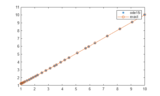
The exact solution of this ODE is
.
Plot the numerical solution y computed by ode15i against the analytical solution ytrue.
ytrue = sqrt(t.^2 + 0.5);
plot(t,y,'*',t,ytrue,'-o')
legend('ode15i', 'exact')
This example reformulates a system of ODEs as a fully implicit system of differential algebraic equations (DAEs). The Robertson problem coded by hb1ode.m is a classic test problem for programs that solve stiff ODEs. The system of equations is

hb1ode solves this system of ODEs to steady state with the initial conditions  ,
,  , and
, and  . But the equations also satisfy a linear conservation law,

In terms of the solution and initial conditions, the conservation law is

The problem can be rewritten as a system of DAEs by using the conservation law to determine the state of  . This reformulates the problem as the implicit DAE system

The function robertsidae encodes this DAE system.
function res = robertsidae(t,y,yp)
res = [yp(1) + 0.04*y(1) - 1e4*y(2)*y(3);
   yp(2) - 0.04*y(1) + 1e4*y(2)*y(3) + 3e7*y(2)^2;
   y(1) + y(2) + y(3) - 1];
The full example code for this formulation of the Robertson problem is available in ihb1dae.m.
Set the error tolerances and the value of  .
.
options = odeset('RelTol',1e-4,'AbsTol',[1e-6 1e-10 1e-6], ...
   'Jacobian',{[],[1 0 0; 0 1 0; 0 0 0]});
Use decic to compute consistent initial conditions from guesses. Fix the first two components of y0 to get the same consistent initial conditions as found by ode15s in hb1dae.m, which formulates this problem as a semi-explicit DAE system.
y0 = [1; 0; 1e-3];
yp0 = [0; 0; 0];
[y0,yp0] = decic(@robertsidae,0,y0,[1 1 0],yp0,[],options);
Solve the system of DAEs using ode15i.
tspan = [0 4*logspace(-6,6)];
[t,y] = ode15i(@robertsidae,tspan,y0,yp0,options);
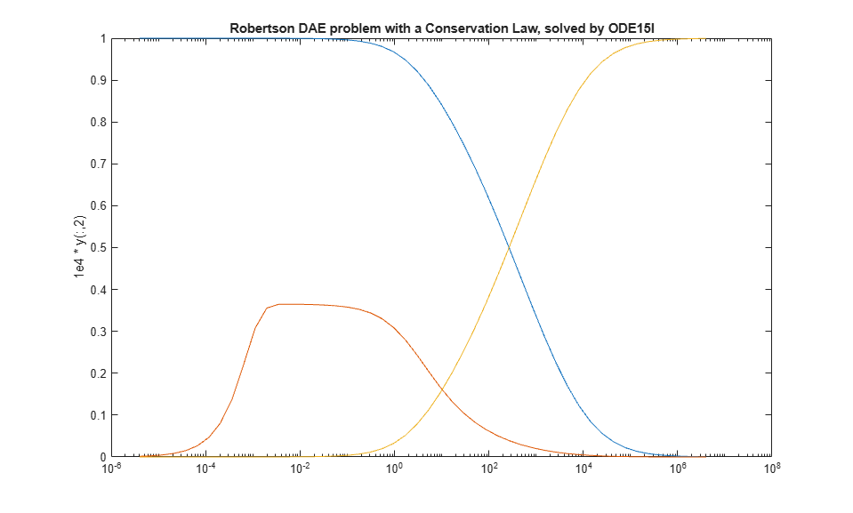
Plot the solution components. Since the second solution component is small relative to the others, multiply it by 1e4 before plotting.
y(:,2) = 1e4*y(:,2);
semilogx(t,y)
ylabel('1e4 * y(:,2)')
title('Robertson DAE problem with a Conservation Law, solved by ODE15I')
Input Arguments
Output Arguments
Tips
Providing the Jacobian matrix to
ode15iis critical for reliability and efficiency. Alternatively, if the system is large and sparse, then providing the Jacobian sparsity pattern also assists the solver. In either case, useodesetto pass in the matrices using theJacobianorJPatternoptions.
Algorithms
ode15i is a variable-step, variable-order
(VSVO) solver based on the backward differentiation formulas (BDFs)
of orders 1 to 5. ode15i is designed to be used
with fully implicit differential equations and index-1 differential
algebraic equations (DAEs). The helper function decic computes
consistent initial conditions that are suitable to be used with ode15i [1].
References
[1] Lawrence F. Shampine, “Solving 0 = F(t, y(t), y′(t)) in MATLAB,” Journal of Numerical Mathematics, Vol.10, No.4, 2002, pp. 291-310.
Version History
Introduced before R2006a