The Apollo 11 Moon Landing: Spacecraft Design Then and Now
By Richard J. Gran and Ossi Saarela, MathWorks
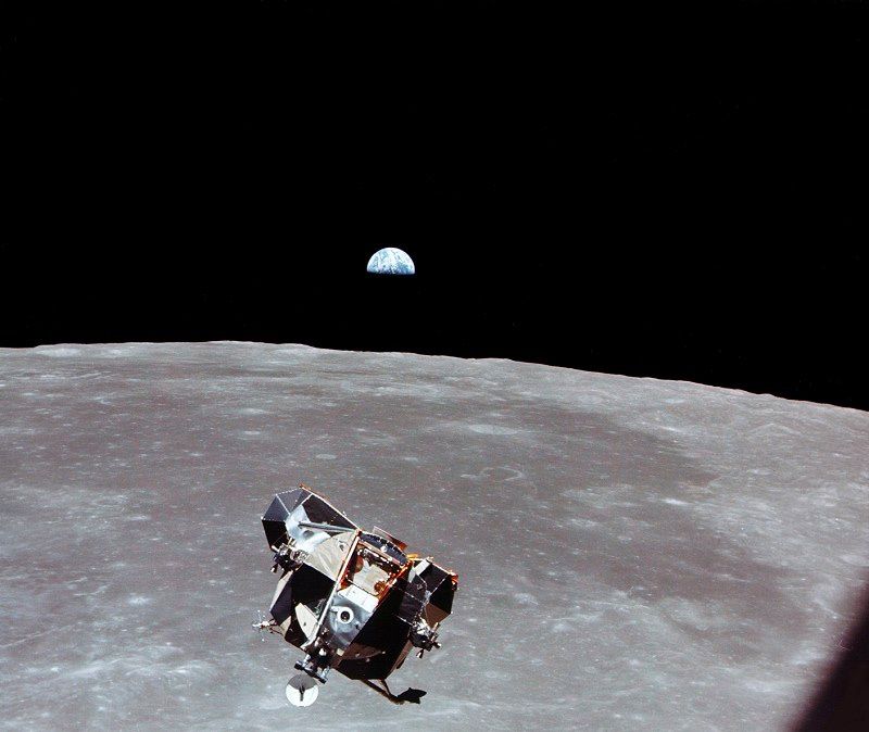
Image courtesy NASA.
Apollo 11, carrying astronauts Neil Armstrong and Buzz Aldrin, landed on the moon over 50 years ago. To commemorate that momentous event, and to celebrate current programs working on the next moon landings, we revisit Richard J. Gran’s firsthand account of designing the Lunar Module digital autopilot, published in 1999. In that article, Richard described the approach he used in the 1960s and compared it with the way Model-Based Design with MATLAB® and Simulink® could be used to design GN&C systems in 1999. In the 20 years since Richard wrote his article, Model-Based Design has evolved significantly. To highlight this evolution, we describe how MATLAB and Simulink can be applied to GN&C system design today.
Richard’s account follows.
As a young boy I always knew I wanted to be an engineer. What I didn't know was that shortly after graduating from college, I would become involved in one of the greatest engineering projects ever. On September 12, 1962, President John F. Kennedy declared, “We choose to go to the Moon in this decade,” setting this nation on an accelerated path to landing a man on the Moon. That same year, I became a member of the Grumman Guidance and Control group, and from 1963 to 1966, participated in the design of the Lunar Module (LM) digital autopilot at Massachusetts Institute of Technology Instrumentation Laboratories (MIT IL).
The Lunar Module Digital Autopilot Design, 1961–1969
The original autopilot proposed for the LM was an analog system that used a modulator to pulse the reaction control jets on and off. While the control system was analog, the navigation and guidance functions ran on a digital computer that was also used by the Command and Service Module (CSM) and the Apollo Booster. The algorithms for guidance and navigation were created by a team at MIT IL, now called Draper Labs.
Early in the Apollo program, NASA decided to enhance mission reliability by programming the Guidance and Navigation Computer to serve as a backup control system for the LM. To do this, a design competition among three of the Apollo contractors (Grumman, MIT IL, and BellComm) was begun in early 1963.
The main issues with the digital autopilot design were its computer speed and storage limits. Roughly 2000 16-bit instructions were allocated to the digital autopilot, and these operations could not interfere with the primary guidance and navigation functions. Among the many problems that had to be solved was the fact that the computer was not designed to process time-critical events. For this reason, there was only one interrupt level, and there were no digital-to-analog interfaces.
To give a feel for how simple this computer was, Table 1 shows the entire set of its operation codes. To implement the digital autopilot, a second interrupt was required. We used the ones-complement structure of the computer, which meant that there was both a positive zero and a negative zero. This allowed a different interrupt to occur when a counter was incremented from a negative number or decremented from a positive number.

Table 1. The operation codes (instructions) available in the Lunar Module guidance computer. The LM guidance computer had eight 4-bit (one-byte) instructions defined by the octal numbers 0–7. A second set of codes (called extend instructions) were available by wasting one machine cycle to indicate that the next op code was from the extended set. Most of the instructions used more than one 12-microsecond machine cycle.
Proposing an Optimal Control System
In 1962, “modern control theory” was still an academic pursuit. There were no textbooks on optimal control. Recent graduates, including me, were not yet versed in state-space methods, and certainly had not been exposed to optimal bang-bang control systems. Engineers at MIT IL worked very closely with students at MIT, and as a consequence, were early adopters of state-space modeling and optimal control techniques based on Pontryagin's Maximum Principle. One of the engineers at MIT IL, George Cherry, proposed using an optimal control system for controlling the vehicle. A spacecraft in space is subject to few external disturbances, which means that the dynamics of its rotational motion can be predicted almost exactly. This near-perfect knowledge of the dynamics gave Cherry the unique insight that the controller could be designed to run at a very slow sample rate.
At the NASA meeting where each design team presented its approach, George Cherry invoked the image of Sir Isaac Newton standing by his side and telling the controller what to do. Needless to say, NASA selected the MIT design. That decision was the right one. The Grumman design required a sample time of .02 seconds or faster, whereas the MIT approach (with Newton's help) only required a sample time of 0.2 seconds (10 times slower than Grumman's design). NASA was so impressed by this structure that they decided not only to implement this LM autopilot but to make it the primary system and relegate the analog system to backup.
The Optimal Controller
The optimal controller developed by Cherry minimized a weighted mix of time and fuel. This theory was described in a book by Athans and Falb1, available in manuscript form. The book was not published until 1966.
Figure 1 shows the logic for firing the reaction control jets programmed into the LM. The parabolas in the figure are the “switch curves” that determine when the reaction jets are turned on and off. The frequency at which the measurements are made is the difficult part of the design.

Figure 1. The reaction control jet phase plane switching logic used in the Lunar Module.
Computer speed and storage limits imposed severe constraints. For example, most control systems engineers would implement this controller by looking at the attitude and rate at some fast sample time to decide where the system currently was in the phase plane. In fact, this is the way the autopilot was implemented when the space shuttle was designed. However, the computer constraints on the LM meant that this strategy would not work, since there was not enough processing power to allow fast sample rates.
Coding and Calculating by Hand
Many processes that are tools of the trade for today's software developer did not exist in 1963. As a consequence, they had to be invented. These processes were often self-imposed disciplines that made the designer's life easier.
One of the first tasks I was given at MIT IL was to develop logic for selecting the appropriate reaction control jets. The code represented by the flow chart in Figure 2 shows self-imposed disciplines that I used to develop this logic. Each path in the code was timed by hand, and both the number of instructions executed and the timing for each branch were calculated using the nominal cycle times for each instruction. Each of the interrupt processing task-timing numbers was also calculated by hand. The flow chart in Figure 2 is a section of the actual computer code in assembly language that took over a year to develop.

Figure 2. Original flowchart from 1966 showing the software design for a piece of the jet select logic code written in assembly language.
The control system design was developed and tested using a simulation written in Fortran at Grumman and in a language called MAC at MIT. Once the design was frozen, the assembly language code was written. This code was then tested in a simulation that emulated the actual computer. This simulation used the assembly language code. To show just how cumbersome the process was: a single “computer run” took half a day. I would typically submit a run in the late afternoon (using IBM cards) and get the results back at 3:00 the following morning. Often, I would get up in the middle of the night and walk from my hotel to MIT IL to fix errors. The results were always in the form of a 10-inch-thick stack of paper with the results of the calculations at each step in the execution of the code.
One reason why the code segment shown in Figure 2 was so complex is that the number of jets that could be used to control the rotations about the pilot axes was large. A decision was made to change the axes that the autopilot was controlling to the “jet axes” shown in Figure 3. This change dramatically reduced the number of lines of code and made it much easier to program the autopilot in the existing computer. Without this improvement, it would have been impossible to have the autopilot use only 2000 words of storage. The lesson of this change is that when engineers are given the opportunity to code the computer with the system they are designing, they can often modify the design to greatly improve the code.
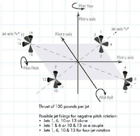
Figure 3. The 16 reaction jets on the Lunar Module as they were positioned relative to the pilot.
Working on the design of the Lunar Module digital autopilot was the highlight of my career as an engineer. When Neil Armstrong stepped off the LM onto the Moon's surface, every engineer who contributed to the Apollo program felt a sense of pride and accomplishment. We had developed technology that never existed before, and through hard work and meticulous attention to detail, we had created a system that worked flawlessly.
How Would the Lunar Module Digital Autopilot Be Designed Today?
Decades after his control design landed Apollo 11 on the Moon, Richard Gran had the opportunity to revisit the LM digital autopilot. This time, he used a Simulink system model. Figure 4 shows what this model would look like today.

Figure 4. Top-level Simulink model of the Lunar Module digital autopilot. The LM rotational dynamics were modeled in about an hour, a fraction of the time it took for the original design. This model can serve multiple functions, including simulation, analysis, and code generation.
In the 1960s, designs were literally drawn on paper. Mathematical calculations were computed by hand, and the implementation was manually coded in assembly language. Today, aerospace engineers use executable models instead of paper designs to abstract the low-level code—an important consideration when designing complex systems. Figure 5 shows a portion of the LM autopilot yaw control law within a Simulink model, implemented using state charts. The embedded source code is generated automatically from the design model, maintaining a direct correlation between design and code.

Figure 5. A portion of the LM autopilot yaw control law. The control law is implemented in Simulink and Stateflow, enabling engineers to work with executable finite state machines instead of writing the textual code. The source code, shown next to the state machine, is automatically generated from the model and includes traceability to the model components (highlighted in blue).
Pressing Play in the LM autopilot Simulink model initiates a simulation that completes in seconds rather than hours, highlighting an important difference between the 1960s and today: the exponential increase in computing speed and power. The role of computer simulation has expanded correspondingly. Thanks to the computing speed now available to them, engineers can simulate many more scenarios than previously, despite the increased complexity of current designs. Through more simulation, expensive hardware tests can be reduced.
Simulation is important, but it is only as useful as the insight into the design that it provides. Not only has simulation speed improved dramatically, so have the speed and ease of analyzing the results. During the Apollo days, it could take hours to pore over paper documents after a simulation completed. Now, engineers have access to parameters, plots, and animations during run time, providing immediate results (Figure 6). Test case execution, postprocessing, and reporting are all automated.

Figure 6. A phase plane plot for the yaw axis control. This plot updates in real time when the simulation is running, providing immediate feedback about the behavior of the control law.
If engineers find unexpected behavior while analyzing the results, design changes may be necessary. In the days of Apollo, it could take days to make a change, analyze its impact, rewrite the code, and resimulate the design. Today, engineering teams using Model-Based Design can contribute changes to their respective portions of the model and immediately simulate the model to see how their changes affect the system. The simulations can run with the model-in-the-loop, software-in-the-loop, or hardware-in-the-loop, depending on the design phase. Dependencies are automatically tracked, eliminating manual tracing, and configuration management tools track changes to the requirements, design, and test cases.
Spacecraft design has always been hard, and today’s computers and software do not eliminate design complexity. However, as the LM autopilot example shows, they can make designs easier to manage, more efficient to test, and quicker to implement, as well as giving the team more time for verification and validation tasks than was possible in the days of Apollo.
We end with Richard Gran’s own observations about Model-Based Design.
“Recreating the digital autopilot design using MATLAB and Simulink brought back memories of the struggles we went through to create the original design. It also emphasized how much better the design process is today: Computer performance is orders of magnitude better, and designing a system with Model-Based Design is far easier. A surprising attribute of today's process is the tight integration of conceptualizing and computing. Because I was able to conceptualize an approach and immediately see if it had merit, I was able to redo the entire LM digital autopilot design in about a week. The analysis, simulation, and testing blend into a seamless procedure. This, in my mind, is the power of Model-Based Design.”
1 Athans, Michael and Peter L. Falb, Optimal Control: An Introduction to the Theory and Its Applications, McGraw-Hill, New York, NY, 1966.
Published 2019
References
-
Gran, Richard, Numerical Computing with Simulink, Volume 1, pp. 94–113, Society for Industrial and Applied Mathematics (SIAM), Philadelphia, PA, 2007.
-
-
Hall, Eldon, Journey to the Moon: The History of the Apollo Guidance Computer, AIAA Press, Reston, VA, 1996.