QPSK and OFDM with MATLAB
This example shows how to simulate a basic communications system that modulates a signal using quadrature phase shift keying (QPSK) and then subjects it to orthogonal frequency division multiplexing (OFDM). It then passes the signal through an additive white Gaussian noise channel before demultiplexing and demodulating the signal. Finally, the system calculates the number of bit errors. To model the system, this example showcases the use of the MATLAB® System object™.
Set the simulation parameters.
M = 4;                 % Modulation alphabet
k = log2(M);           % Bits/symbol
numSC = 128;           % Number of OFDM subcarriers
cpLen = 32;            % OFDM cyclic prefix length
maxBitErrors = 100;    % Maximum number of bit errors
maxNumBits = 1e7;      % Maximum number of bits transmitted
Construct System objects for the simulation: an OFDM modulator, an OFDM demodulator, and an error rate calculator. Use name-value arguments to set the object properties.
Set the OFDM modulator and demodulator pair according to the simulation parameters. You must use a System object for OFDM windowing because applying the technique at one symbol requires information about the samples of the previous symbol. The System object saves this information as an internal state. For more information, see OFDM Raised Cosine Windowing.
ofdmMod = comm.OFDMModulator( ...
    FFTLength=numSC, ...
    CyclicPrefixLength=cpLen, ...
    Windowing=true, ...
    WindowLength=16);
ofdmDemod = comm.OFDMDemodulator( ...
    FFTLength=numSC, ...
    CyclicPrefixLength=cpLen);
Create the error rate calculator. Set the ResetInputPort property to true so that it can be reset during the simulation.
errorRate = comm.ErrorRate(ResetInputPort=true);
To determine the input and output dimensions of the OFDM modulator, use the info function of the ofdmMod object
ofdmDims = info(ofdmMod)
ofdmDims = struct with fields:
    DataInputSize: [117 1]
       OutputSize: [160 1]
Determine the number of data subcarriers from the ofdmDims structure variable.
numDC = ofdmDims.DataInputSize(1)
numDC =
117
Determine the OFDM frame size (in bits) from the number of data subcarriers and the number of bits per symbol.
frameSize = [k*numDC 1];
Set the SNR vector based on the desired Eb/No range, the number of bits per symbol, and the ratio of the number of data subcarriers to the total number of subcarriers.
EbNoVec = (0:10)';
snrVec = EbNoVec + 10*log10(k) + 10*log10(numDC/numSC);
Initialize the BER and error statistics arrays.
berVec = zeros(length(EbNoVec),3);
errorStats = zeros(1,3);
Simulate the communication link over the range of Eb/No values. For each Eb/No value, the simulation runs until the system records maxBitErrors or the total number of transmitted bits exceeds maxNumBits.
for m = 1:length(EbNoVec)
    snr = snrVec(m);

   while errorStats(2) <= maxBitErrors && errorStats(3) <= maxNumBits
       dataIn = randi([0,1],frameSize);
       qpskTx = pskmod(dataIn,M,InputType="bit");
       txSig = ofdmMod(qpskTx);
       powerDB = 10*log10(var(txSig));
       noiseVar = 10.^(0.1*(powerDB-snr));
       noise = sqrt(noiseVar/2)*complex(randn(size(txSig)), ...
           randn(size(txSig)));
       rxSig = txSig + noise;
       qpskRx = ofdmDemod(rxSig);
       dataOut = pskdemod(qpskRx,M,OutputType="bit");
       errorStats = errorRate(dataIn,dataOut,0);
   end

    berVec(m,:) = errorStats;
    errorStats = errorRate(dataIn,dataOut,1);
end
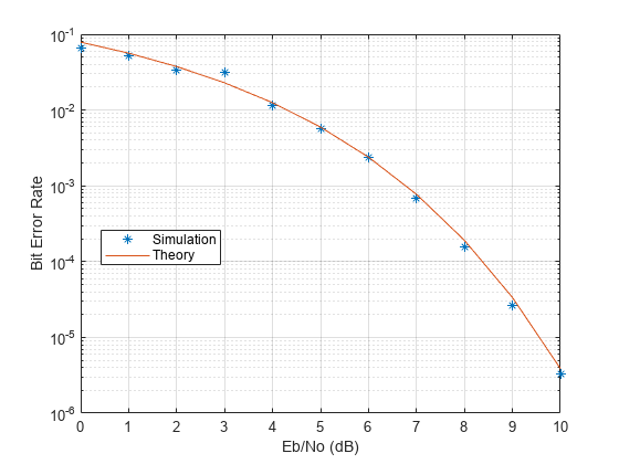
To determine the theoretical BER for a QPSK system, use the berawgn function.
berTheory = berawgn(EbNoVec,'psk',M,'nondiff');
To compare result, plot the theoretical and simulated data on the same graph.
figure
semilogy(EbNoVec,berVec(:,1),'*')
hold on
semilogy(EbNoVec,berTheory)
legend('Simulation','Theory','Location','Best')
xlabel('Eb/No (dB)')
ylabel('Bit Error Rate')
grid on
hold off