Simulate GARCH Models
This example shows how to simulate from a GARCH process with and without specifying presample data. The sample unconditional variances of the Monte Carlo simulations approximate the theoretical GARCH unconditional variance.
Step 1. Specify a GARCH model.
Specify a GARCH(1,1) model where the distribution of is Gaussian and
Mdl = garch('Constant',0.01,'GARCH',0.7,'ARCH',0.25)
Mdl =
  garch with properties:

     Description: "GARCH(1,1) Conditional Variance Model (Gaussian Distribution)"
      SeriesName: "Y"
    Distribution: Name = "Gaussian"
               P: 1
               Q: 1
        Constant: 0.01
           GARCH: {0.7} at lag [1]
            ARCH: {0.25} at lag [1]
          Offset: 0
Step 2. Simulate from the model without using presample data.
Simulate five paths of length 100 from the GARCH(1,1) model, without specifying any presample innovations or conditional variances. Display the first conditional variance for each of the five sample paths. The model being simulated does not have a mean offset, so the response series is an innovation series.
rng default; % For reproducibility
[Vn,Yn] = simulate(Mdl,100,'NumPaths',5);

Vn(1,:) % Display variances
ans = 1×5

    0.1645    0.3182    0.4051    0.1872    0.1551
figure
subplot(2,1,1)
plot(Vn)
xlim([0,100])
title('Conditional Variances')

subplot(2,1,2)
plot(Yn)
xlim([0,100])
title('Innovations')
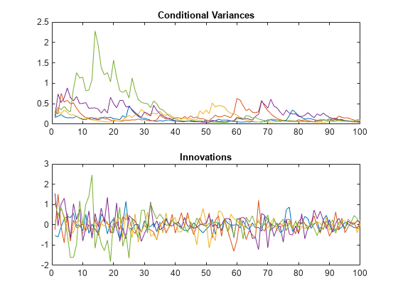
The starting conditional variances are different for each realization because no presample data was specified.
Step 3. Simulate from the model using presample data.
Simulate five paths of length 100 from the model, specifying the one required presample innovation and conditional variance. Display the first conditional variance for each of the five sample paths.
rng default;
[Vw,Yw] = simulate(Mdl,100,'NumPaths',5,...
    'E0',0.05,'V0',0.001);

Vw(1,:)
ans = 1×5

    0.0113    0.0113    0.0113    0.0113    0.0113
figure
subplot(2,1,1)
plot(Vw)
xlim([0,100])
title('Conditional Variances')

subplot(2,1,2)
plot(Yw)
xlim([0,100])
title('Innovations')
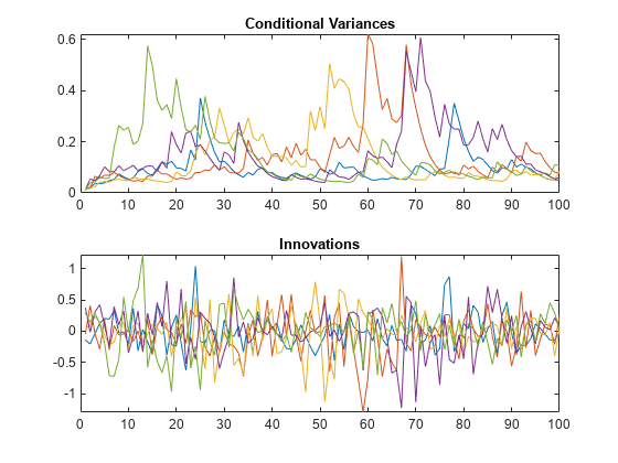
All five sample paths have the same starting conditional variance, calculated using the presample data.
Note that even with the same starting variance, the realizations of the innovation series have different starting points. This is because each is a random draw from a Gaussian distribution with mean 0 and variance .
Step 4. Look at the unconditional variances.
Simulate 10,000 sample paths of length 500 from the specified GARCH model. Plot the sample unconditional variances of the Monte Carlo simulations, and compare them to the theoretical unconditional variance,
sig2 = 0.01/(1-0.7-0.25);

rng default;
[V,Y] = simulate(Mdl,500,'NumPaths',10000);

figure
plot(var(Y,0,2),'Color',[.7,.7,.7],'LineWidth',1.5)
xlim([0,500])
hold on
plot(1:500,ones(500,1)*sig2,'k--','LineWidth',2)
legend('Simulated','Theoretical','Location','NorthWest')
title('Unconditional Variance')
hold off
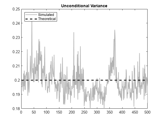
The simulated unconditional variances fluctuate around the theoretical unconditional variance.