sdeld
SDE with Linear Drift (SDELD) model
Description
Creates and displays a SDE object whose drift rate is expressed in linear
drift-rate form and that derives from the sdeddo (SDE from drift and diffusion objects class).
Use sdeld objects to simulate sample paths of
NVars state variables expressed in linear drift-rate form. They
provide a parametric alternative to the mean-reverting drift form (see sdemrd).
These state variables are driven by NBrowns Brownian motion sources
of risk over NPeriods consecutive observation periods, approximating
continuous-time stochastic processes with linear drift-rate functions.
The sdeld object allows you to simulate any vector-valued SDELD of
the form:
where:
Xt is an
NVars-by-1state vector of process variables.A is an
NVars-by-1vector.B is an
NVars-by-NVarsmatrix.D is an
NVars-by-NVarsdiagonal matrix, where each element along the main diagonal is the corresponding element of the state vector raised to the corresponding power of α.V is an
NVars-by-NBrownsinstantaneous volatility rate matrix.dWt is an
NBrowns-by-1Brownian motion vector.
Creation
Description
SDELD = sdeld(___,Name,Value)SDELD object with additional options specified
by one or more Name,Value pair arguments.
Name is a property name and Value is
its corresponding value. Name must appear inside single
quotes (''). You can specify several name-value pair
arguments in any order as
Name1,Value1,…,NameN,ValueN.
The SDELD object has the following displayed Properties:
StartTime— Initial observation timeStartState— Initial state at timeStartTimeCorrelation— Access function for theCorrelationinput argument, callable as a function of timeDrift— Composite drift-rate function, callable as a function of time and stateDiffusion— Composite diffusion-rate function, callable as a function of time and stateA— Access function for the input argumentA, callable as a function of time and stateB— Access function for the input argumentB, callable as a function of time and stateAlpha— Access function for the input argumentAlpha, callable as a function of time and stateSigma— Access function for the input argumentSigma, callable as a function of time and stateSimulation— A simulation function or method
Input Arguments
Properties
Object Functions
interpolate | Brownian interpolation of stochastic differential equations (SDEs) for
SDE, BM, GBM,
CEV, CIR, HWV,
Heston, SDEDDO, SDELD, or
SDEMRD models |
simulate | Simulate multivariate stochastic differential equations (SDEs) for
SDE, BM, GBM,
CEV, CIR, HWV,
Heston, SDEDDO, SDELD,
SDEMRD, Merton, or Bates
models |
simByEuler | Euler simulation of stochastic differential equations (SDEs) for
SDE, BM, GBM,
CEV, CIR, HWV,
Heston, SDEDDO, SDELD, or
SDEMRD models |
simByMilstein | Simulate diagonal diffusion for BM, GBM,
CEV, HWV, SDEDDO,
SDELD, or SDEMRD sample paths by Milstein
approximation |
simByMilstein2 | Simulate BM, GBM, CEV,
HWV, SDEDDO, SDELD,
SDEMRD process sample paths by second order Milstein
approximation |
Examples
More About
Instance Hierarchy
There are inheritance relationships among the SDE classes.
The following figure illustrates the inheritance relationships.
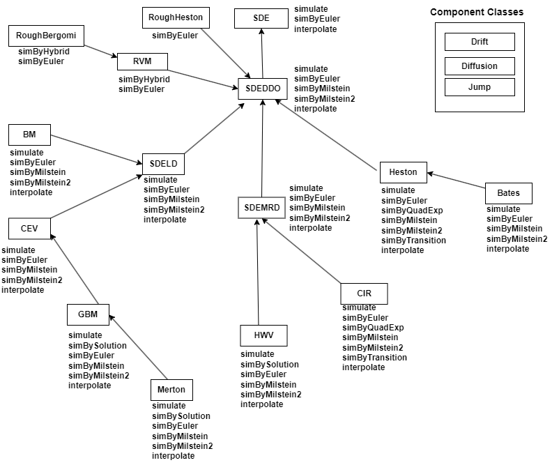
For more information, see SDE Class Hierarchy.
Algorithms
When you specify the required input parameters as arrays, they are associated with a specific parametric form. By contrast, when you specify either required input parameter as a function, you can customize virtually any specification.
Accessing the output parameters with no inputs simply returns the original input specification. Thus, when you invoke these parameters with no inputs, they behave like simple properties and allow you to test the data type (double vs. function, or equivalently, static vs. dynamic) of the original input specification. This is useful for validating and designing methods.
When you invoke these parameters with inputs, they behave like functions, giving the
impression of dynamic behavior. The parameters accept the observation time
t and a state vector
Xt, and return an array of appropriate
dimension. Even if you originally specified an input as an array,
sdeld treats it as a static function of time and state, by that
means guaranteeing that all parameters are accessible by the same interface.
References
[1] Aït-Sahalia, Yacine. “Testing Continuous-Time Models of the Spot Interest Rate.” Review of Financial Studies, vol. 9, no. 2, Apr. 1996, pp. 385–426.
[2] Aït-Sahalia, Yacine. “Transition Densities for Interest Rate and Other Nonlinear Diffusions.” The Journal of Finance, vol. 54, no. 4, Aug. 1999, pp. 1361–95.
[3] Glasserman, Paul. Monte Carlo Methods in Financial Engineering. Springer, 2004.
[4] Hull, John. Options, Futures and Other Derivatives. 7th ed, Prentice Hall, 2009.
[5] Johnson, Norman Lloyd, et al. Continuous Univariate Distributions. 2nd ed, Wiley, 1994.
[6] Shreve, Steven E. Stochastic Calculus for Finance. Springer, 2004.
Version History
Introduced in R2008aSee Also
drift | diffusion | sdeddo | simByEuler | nearcorr
Topics
- Linear Drift Models
- Implementing Multidimensional Equity Market Models, Implementation 3: Using SDELD, CEV, and GBM Objects
- Simulating Equity Prices
- Simulating Interest Rates
- Stratified Sampling
- Price American Basket Options Using Standard Monte Carlo and Quasi-Monte Carlo Simulation
- Base SDE Models
- Drift and Diffusion Models
- Linear Drift Models
- Parametric Models
- SDEs
- SDE Models
- SDE Class Hierarchy
- Quasi-Monte Carlo Simulation
- Performance Considerations
You can also select a web site from the following list:
Americas
- América Latina (Español)
- Canada (English)
- United States (English)
Europe
- Belgium (English)
- Denmark (English)
- Deutschland (Deutsch)
- España (Español)
- Finland (English)
- France (Français)
- Ireland (English)
- Italia (Italiano)
- Luxembourg (English)
- Netherlands (English)
- Norway (English)
- Österreich (Deutsch)
- Portugal (English)
- Sweden (English)
- Switzerland
- United Kingdom (English)