Convert Fast Fourier Transform (FFT) to Fixed Point
This example shows how to convert a textbook version of the Fast Fourier Transform (FFT) algorithm into fixed-point MATLAB® code.
Textbook FFT Algorithm
FFT is a complex-valued linear transformation from the time domain to the frequency domain. For example, if you construct a vector as the sum of two sinusoids and transform it with the FFT, you can see the peaks of the frequencies in the FFT magnitude plot.
n = 64;                                     % Number of points
Fs = 4;                                     % Sampling frequency in Hz
t  = (0:(n-1))/Fs;                          % Time vector
f  = linspace(0,Fs,n);                      % Frequency vector
f0 = 0.2; f1 = 0.5;                         % Frequencies, in Hz
x0 = cos(2*pi*f0*t) + 0.55*cos(2*pi*f1*t);  % Time-domain signal
x0 = complex(x0);                           % The textbook algorithm requires the input to be complex
y0  = fft(x0);                              % Frequency-domain transformation fft() is a MATLAB built-in function

fi_fft_demo_ini_plot(t,x0,f,y0);            % Plot the results from fft and time-domain signal
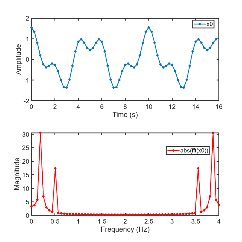
The peaks at 0.2 and 0.5 Hz in the frequency plot correspond to the two sinusoids of the time-domain signal at those frequencies.
Note the reflected peaks at 3.5 and 3.8 Hz. When the input to an FFT is real-valued, as it is in this case, then the output is the conjugate-symmetric:
There are many different implementations of the FFT, each having its own costs and benefits. You may find that a different algorithm is better for your application than the one given here. This algorithm provides you with an example of how you can begin your own exploration.
This example uses the decimation-in-time unit-stride FFT shown in Algorithm 1.6.2 on page 45 of the book Computational Frameworks for the Fast Fourier Transform by Charles Van Loan.
In pseudo-code, the algorithm in the textbook is as follows:
Algorithm 1.6.2. If is a complex vector of length and , then the following algorithm overwrites with .
(See Van Loan section 1.4.11.)
for
for
for
end
end
end
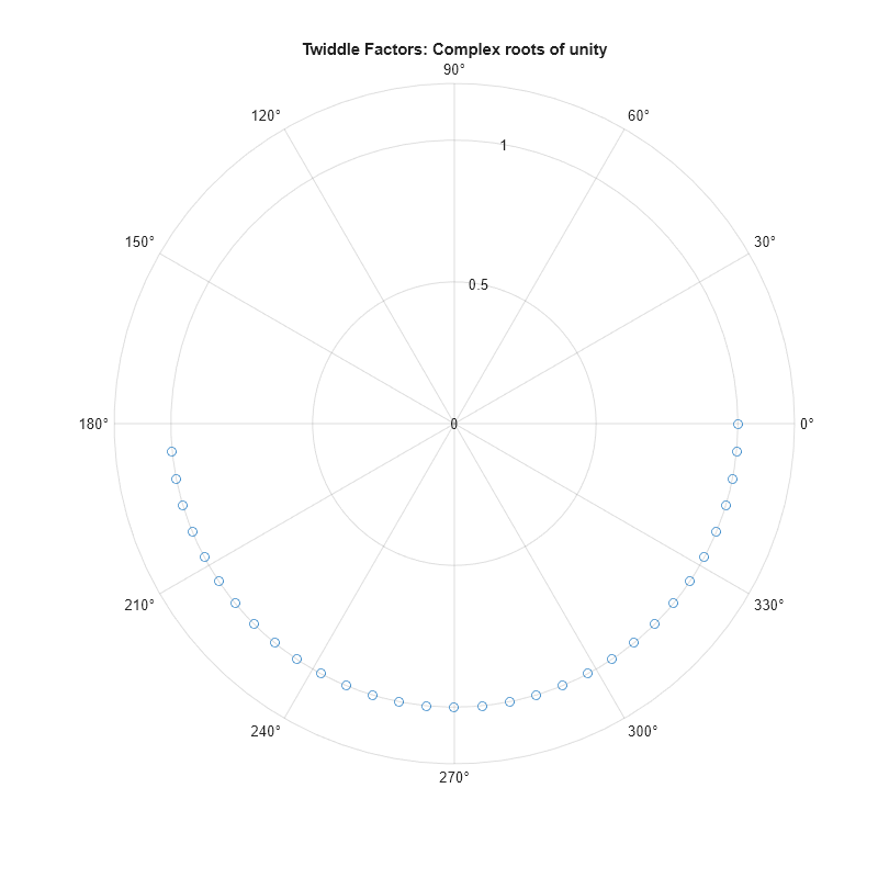
The textbook algorithm uses zero-based indexing. is an n-by-n Fourier-transform matrix, is an n-by-n bit-reversal permutation matrix, and is a complex vector of twiddle factors. The twiddle factors, , are complex roots of unity computed by the following algorithm:
function w = fi_radix2twiddles(n)
%FI_RADIX2TWIDDLES  Twiddle factors for radix-2 FFT example.
%   W = FI_RADIX2TWIDDLES(N) computes the length N-1 vector W of
%   twiddle factors.

%   Reference:
%
%   Twiddle factors for Algorithm 1.6.2, p. 45, Charles Van Loan,
%   Computational Frameworks for the Fast Fourier Transform, SIAM,
%   Philadelphia, 1992.
%
%   Copyright 2003-2011 The MathWorks, Inc.
%

t = log2(n);
if floor(t) ~= t
  error('N must be an exact power of two.');
end

w = zeros(n-1,1);
k = 1;
L = 2;
% Equation 1.4.11, p. 34
while L <= n
  theta = 2*pi/L;
  % Algorithm 1.4.1, p. 23
  for j = 0:(L/2 - 1)
    w(k) = complex(cos(j*theta),-sin(j*theta));
    k = k + 1;
  end
  L = L*2;
end
figure(gcf)
clf
w0 = fi_radix2twiddles(n);
polarplot(angle(w0),abs(w0),'o')
title('Twiddle Factors: Complex roots of unity')
Verify Floating-Point Code
To implement the algorithm in MATLAB®, you can use the fi_bitreverse function to bit-reverse the input sequence. You must add one to the indices to convert them from zero-based to one-based.
function x = fi_m_radix2fft_algorithm1_6_2(x, w)
%FI_M_RADIX2FFT_ALGORITHM1_6_2  Radix-2 FFT example.
%   Y = FI_M_RADIX2FFT_ALGORITHM1_6_2(X, W) computes the radix-2 FFT of
%   input vector X with twiddle-factors W.  Input X is assumed to be
%   complex.
%
%   The length of vector X must be an exact power of two.
%   Twiddle-factors W are computed via
%      W = fi_radix2twiddles(N)
%   where N = length(X).
%
%   This version of the algorithm has no scaling before the stages.

%   Reference:
%     Charles Van Loan, Computational Frameworks for the Fast Fourier
%     Transform, SIAM, Philadelphia, 1992, Algorithm 1.6.2, p. 45.
%
%   Copyright 2004-2015 The MathWorks, Inc.

    n = length(x);  t = log2(n);
    x = fi_bitreverse(x,n);
    for q=1:t
        L = 2^q; r = n/L; L2 = L/2;
        for k = 0:(r-1)
            for j = 0:(L2-1)
                temp          = w(L2-1+j+1) * x(k*L+j+L2+1);
                x(k*L+j+L2+1) = x(k*L+j+1)  - temp;
                x(k*L+j+1)    = x(k*L+j+1)  + temp;
            end
        end
    end
end
Visualization
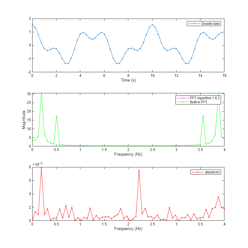
To verify that you correctly implemented the algorithm in MATLAB®, run a known signal through it and compare the results to the results produced by the MATLAB® FFT function.
As seen in the plot below, the error is within tolerance of the MATLAB® built-in FFT function, verifying that you have correctly implemented the algorithm.
y = fi_m_radix2fft_algorithm1_6_2(x0, w0);

fi_fft_demo_plot(real(x0),y,y0,Fs,'Double data', ...
    {'FFT Algorithm 1.6.2','Built-in FFT'});
Convert Functions to Use Types Tables
To separate data types from the algorithm:
Create a table of data type definitions.
Modify the algorithm code to use data types from that table.
This example shows the iterative steps by creating different files. In practice, you can make the iterative changes to the same file.
Original types table
Create a types table using a structure with prototypes for the variables set to their original types. Use the baseline types to validate that you made the initial conversion correctly, and to programmatically toggle your function between floating point and fixed point types. The index variables are automatically converted to integers by MATLAB® Coder™, so you don't need to specify their types in the table.
Specify the prototype values as empty ([ ]) since the data types are used, but not the values.
function T = fi_m_radix2fft_original_types()

%   Copyright 2015 The MathWorks, Inc.

    T.x = double([]);
    T.w = double([]);
    T.n = double([]);

end
Type-aware algorithm function
Add types table T as an input to the function and use it to cast variables to a particular type, while keeping the body of the algorithm unchanged.
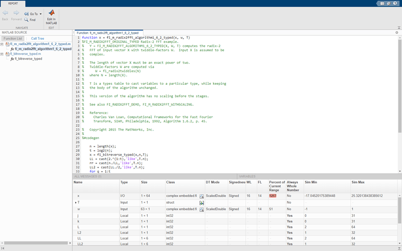
function x = fi_m_radix2fft_algorithm1_6_2_typed(x, w, T)
%FI_M_RADIX2FFT_ORIGINAL_TYPED Radix-2 FFT example.
%   Y = FI_M_RADIX2FFT_ALGORITHM1_6_2_TYPED(X, W, T) computes the radix-2
%   FFT of input vector X with twiddle-factors W.  Input X is assumed to be
%   complex.
%
%   The length of vector X must be an exact power of two.
%   Twiddle-factors W are computed via
%      W = fi_radix2twiddles(N)
%   where N = length(X).
%
%   T is a types table to cast variables to a particular type, while keeping
%   the body of the algorithm unchanged.
%
%   This version of the algorithm has no scaling before the stages.
%
%   Reference:
%     Charles Van Loan, Computational Frameworks for the Fast Fourier
%     Transform, SIAM, Philadelphia, 1992, Algorithm 1.6.2, p. 45.

%   Copyright 2015 The MathWorks, Inc.
%
%#codegen

    n = length(x);
    t = log2(n);
    x = fi_bitreverse_typed(x,n,T);
    LL = cast(2.^(1:t),'like',T.n);
    rr = cast(n./LL,'like',T.n);
    LL2 = cast(LL./2,'like',T.n);
    for q=1:t
        L = LL(q);
        r = rr(q);
        L2 = LL2(q);
        for k = 0:(r-1)
            for j = 0:(L2-1)
                temp          = w(L2-1+j+1) * x(k*L+j+L2+1);
                x(k*L+j+L2+1) = x(k*L+j+1)  - temp;
                x(k*L+j+1)    = x(k*L+j+1)  + temp;
            end
        end
    end
end
Type-aware bit-reversal function
Add types table T as an input to the function and use it to cast variables to a particular type, while keeping the body of the algorithm unchanged.
function x = fi_bitreverse_typed(x,n0,T)
%FI_BITREVERSE_TYPED  Bit-reverse the input.
%   X = FI_BITREVERSE_TYPED(x,n,T) bit-reverse the input sequence X, where
%   N=length(X).
%
%   T is a types table to cast variables to a particular type, while keeping
%   the body of the algorithm unchanged.
%

%   Copyright 2004-2015 The MathWorks, Inc.
%
%#codegen
n = cast(n0,'like',T.n);
nv2 = bitsra(n,1);
j = cast(1,'like',T.n);
for i = 1:(n-1)
  if i < j
    temp = x(j);
    x(j) = x(i);
    x(i) = temp;
  end
  k = nv2;
  while k < j
    j(:) = j-k;
    k = bitsra(k,1);
  end
  j(:) = j+k;
end
Validate modified function
Every time you modify your function, validate that the results still match your baseline. Since you used the original types in the types table, the outputs should be identical. This validates that you made the conversion to separate the types from the algorithm correctly.
T1 = fi_m_radix2fft_original_types(); % Get original data types declared in table

x = cast(x0,'like',T1.x);
w = cast(w0,'like',T1.w);

y = fi_m_radix2fft_algorithm1_6_2_typed(x, w, T1);

fi_fft_demo_plot(real(x),y,y0,Fs,'Double data', ...
    {'FFT Algorithm 1.6.2','Built-in FFT'});

Create a Fixed-Point Types Table
Create a fixed-point types table using a structure with prototypes for the variables. Specify the prototype values as empty ([ ]) since the data types are used, but not the values.
function T = fi_m_radix2fft_fixed_types()

%   Copyright 2015 The MathWorks, Inc.

    T.x = fi([],1,16,14); % Picked the following types to ensure that the
    T.w = fi([],1,16,14); % inputs have maximum precision and will not
                          % overflow
    T.n = int32([]);      % Picked int32 as n is an index

end
Identify Fixed-Point Issues
Now, try converting the input data to fixed-point and see if the algorithm still looks good. In this first pass, you use all the defaults for signed fixed-point data by using the fi constructor.
T2 = fi_m_radix2fft_fixed_types(); % Get fixed point data types declared in table

x = cast(x0,'like',T2.x);
w = cast(w0,'like',T2.w);
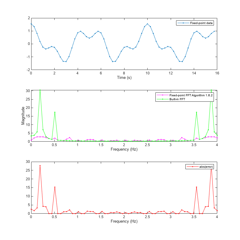
Re-run the same algorithm with the fixed-point inputs.
y  = fi_m_radix2fft_algorithm1_6_2_typed(x,w,T2);
fi_fft_demo_plot(real(x),y,y0,Fs,'Fixed-point data', ...
    {'Fixed-point FFT Algorithm 1.6.2','Built-in FFT'});
Note that the magnitude plot (center) of the fixed-point FFT does not resemble the plot of the built-in FFT. The error (bottom plot) is much larger than what you would expect to see for round off error, so it is likely that overflow has occurred.
Use Min/Max Instrumentation to Identify Overflows
To instrument the MATLAB® code, create a MEX function from the MATLAB® function using the buildInstrumentedMex command. The inputs to buildInstrumentedMex are the same as the inputs to fiaccel, but buildInstrumentedMex has no fi object restrictions. The output of buildInstrumentedMex is a MEX function with instrumentation inserted, so when the MEX function is run, the simulated minimum and maximum values are recorded for all named variables and intermediate values.
The '-o' option is used to name the MEX function that is generated. If the '-o' option is not used, then the MEX function is the name of the MATLAB® function with '_mex' appended. You can also name the MEX function the same as the MATLAB® function, but you need to remember that MEX functions take precedence over MATLAB® functions and so changes to the MATLAB® function will not run until either the MEX function is regenerated, or the MEX function is deleted and cleared.
Create the input with a scaled double data type so its values will attain full range and you can identify potential overflows.
function T = fi_m_radix2fft_scaled_fixed_types()

%   Copyright 2015 The MathWorks, Inc.

    DT = 'ScaledDouble';                % Data type to be used for fi
                                        % constructor
    T.x = fi([],1,16,14,'DataType',DT); % Picked the following types to
    T.w = fi([],1,16,14,'DataType',DT); % ensure that the inputs have
                                        % maximum precision and will not
                                        % overflow
    T.n = int32([]);                    % Picked int32 as n is an index

end
T3 = fi_m_radix2fft_scaled_fixed_types(); % Get fixed point data types declared in table

x_scaled_double = cast(x0,'like',T3.x);
w_scaled_double = cast(w0,'like',T3.w);

buildInstrumentedMex fi_m_radix2fft_algorithm1_6_2_typed ...
    -o fft_instrumented -args {x_scaled_double w_scaled_double T3}
Run the instrumented MEX function to record min/max values.
y_scaled_double = fft_instrumented(x_scaled_double,w_scaled_double,T3);
Show the instrumentation results.
showInstrumentationResults fft_instrumented
You can see from the instrumentation results that there were overflows when assigning into the variable x.
Modify the Algorithm to Address Fixed-Point Issues
The magnitude of an individual bin in the FFT grows, at most, by a factor of n, where n is the length of the FFT. Hence, by scaling your data by 1/n, you can prevent overflow from occurring for any input. When you scale only the input to the first stage of a length-n FFT by 1/n, you obtain a signal-to-noise ratio proportional to n^2 [Oppenheim & Schafer 1989, equation 9.101], [Welch 1969]. However, if you scale the input to each of the stages of the FFT by 1/2, you can obtain an overall scaling of 1/n and produce a signal-to-noise ratio proportional to n [Oppenheim & Schafer 1989, equation 9.105], [Welch 1969].
An efficient way to scale by 1/2 in fixed-point is to right-shift the data. To do this, you use the bit shift right arithmetic function bitsra. After scaling each stage of the FFT, and optimizing the index variable computation, your algorithm becomes:
function x = fi_m_radix2fft_withscaling_typed(x, w, T)
% Radix-2 FFT example with scaling at each stage.
%   Y = FI_M_RADIX2FFT_WITHSCALING_TYPED(X, W, T) computes the radix-2 FFT of
%   input vector X with twiddle-factors W with scaling by 1/2 at each stage.
%   Input X is assumed to be complex.
%
%   The length of vector X must be an exact power of two.
%   Twiddle-factors W are computed via
%      W = fi_radix2twiddles(N)
%   where N = length(X).
%
%   T is a types table to cast variables to a particular type, while keeping
%   the body of the algorithm unchanged.
%
%   This version of the algorithm has no scaling before the stages.
%

%   Reference:
%     Charles Van Loan, Computational Frameworks for the Fast Fourier
%     Transform, SIAM, Philadelphia, 1992, Algorithm 1.6.2, p. 45.
%
%   Copyright 2004-2015 The MathWorks, Inc.
%
%#codegen

    n = length(x);  t = log2(n);
    x = fi_bitreverse(x,n);

    % Generate index variables as integer constants so they are not computed in
    % the loop.
    LL = cast(2.^(1:t),'like',T.n);
    rr = cast(n./LL,'like',T.n);
    LL2 = cast(LL./2,'like',T.n);
    for q = 1:t
        L = LL(q); r = rr(q); L2 = LL2(q);
        for k = 0:(r-1)
            for j = 0:(L2-1)
                temp          = w(L2-1+j+1) * x(k*L+j+L2+1);
                x(k*L+j+L2+1) = bitsra(x(k*L+j+1) - temp, 1);
                x(k*L+j+1)    = bitsra(x(k*L+j+1) + temp, 1);
            end
        end
    end
end
Run the scaled algorithm with fixed-point data.
x = cast(x0,'like',T3.x);
w = cast(w0,'like',T3.w);

y = fi_m_radix2fft_withscaling_typed(x,w,T3);

fi_fft_demo_plot(real(x), y, y0/n, Fs, 'Fixed-point data', ...
    {'Fixed-point FFT with scaling','Built-in FFT'});
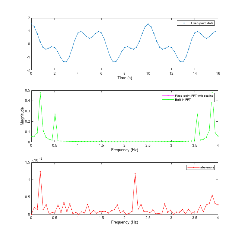
You can see that the scaled fixed-point FFT algorithm now matches the built-in FFT to a tolerance that is expected for 16-bit fixed-point data.
References
Charles Van Loan, Computational Frameworks for the Fast Fourier Transform, SIAM, 1992.
Cleve Moler, Numerical Computing with MATLAB, SIAM, 2004, Chapter 8 Fourier Analysis.
Alan V. Oppenheim and Ronald W. Schafer, Discrete-Time Signal Processing, Prentice Hall, 1989.
Peter D. Welch, "A Fixed-Point Fast Fourier Transform Error Analysis," IEEE® Transactions on Audio and Electroacoustics, Vol. AU-17, No. 2, June 1969, pp. 151-157.
You can also select a web site from the following list:
Americas
- América Latina (Español)
- Canada (English)
- United States (English)
Europe
- Belgium (English)
- Denmark (English)
- Deutschland (Deutsch)
- España (Español)
- Finland (English)
- France (Français)
- Ireland (English)
- Italia (Italiano)
- Luxembourg (English)
- Netherlands (English)
- Norway (English)
- Österreich (Deutsch)
- Portugal (English)
- Sweden (English)
- Switzerland
- United Kingdom (English)