Introduction to Forecasting of Dynamic System Response
Forecasting the response of a dynamic system is the prediction of future outputs of the system using past output measurements. In other words, given observations y(t) = {y(1), …, y(N)} of the output of a system, forecasting is the prediction of the outputs y(N+1), …, y(N+H) until a future time horizon H.
When you perform forecasting in System Identification Toolbox™ software, you first identify a model that fits past measured data from the
system. The model can be a linear time series model such as AR, ARMA, and state-space
models, or a nonlinear ARX model. If exogenous inputs influence the outputs of the
system, you can perform forecasting using input-output models such as ARX and ARMAX.
After identifying the model, you then use the forecast command to compute y(N+1), …,
y(N+H). The command computes the forecasted values by:
Generating a predictor model using the identified model.
Computing the final state of the predictor using past measured data.
Simulating the identified model until the desired forecasting horizon, H, using the final state as initial conditions.
This topic illustrates these forecasting steps for linear and nonlinear models. Forecasting the response of systems without external inputs (time series data) is illustrated, followed by forecasting for systems with an exogenous input. For information about how to perform forecasting in the toolbox, see Forecast Output of Dynamic System.
Forecasting Time Series Using Linear Models
The toolbox lets you forecast time series (output only) data using linear models such as AR, ARMA, and state-space models. Here is an illustration of forecasting the response of an autoregressive model, followed by the forecasting steps for more complex models such as moving-average and state-space models.
Autoregressive Models
Suppose that you have collected time series data y(t) = {y(1), …, y(N)} of a stationary random process. Assuming the data is a second-order autoregressive (AR) process, you can describe the dynamics by the following AR model:
Where a1 and a2 are the fit coefficients and e(t) is the noise term.
You can identify the model using the ar command.
The software computes the fit coefficients and variance of e(t)
by minimizing the 1-step prediction errors between the observations
{y(1), …, y(N)} and model
response.
Assuming that the innovations e(t) are a zero mean white sequence, you can compute the predicted output using the formula:
Where y(t-1) and y(t-2) are either measured data, if available, or previously predicted values. For example, the forecasted outputs five steps in the future are:
Note that the computation of uses the previously predicted value because measured data is not available beyond time step N. Thus, the direct contribution of measured data diminishes as you forecast further into the future.
The forecasting formula is more complex for time series processes that contain moving-average terms.
Moving-Average Models
In moving-average (MA) models, the output depends on current and past innovations (e(t),e(t-1), e(t-2), e(t-3)....). Thus, forecasting the response of MA models requires knowledge of the initial conditions of the measured data.
Suppose that time series data y(t) from your system can be fit to a second-order moving-average model:
Suppose that y(1) and y(2) are
the only available observations, and their values equal 5 and 10,
respectively. You can estimate the model coefficients c1 and c2 using
the armax command. Assume that
the estimated c1 and c2 values
are 0.1 and 0.2, respectively. Then assuming as before that e(t)
is a random variable with zero mean, you can predict the output value
at time t using the following formula:
Where e(t-1) and e(t-2) are
the differences between the measured and the predicted response at
times t-1 and t-2, respectively.
If measured data does not exist for these times, a zero value is used
because the innovations process e(t)
is assumed to be zero-mean white Gaussian noise.
Therefore, forecasted output at time t = 3 is:
Where, the innovations e(1) and e(2) are
the difference between the observed and forecasted values of output
at time t equal to 1 and 2,
respectively:
Because the data was measured from time t equal
to 1, the values of e(0) and e(-1) are
unknown. Thus, to compute the forecasted outputs, the value of these
initial conditions e(0) and e(-1) is
required. You can either assume zero initial conditions, or estimate
them.
Zero initial conditions: If you specify that
e(0)ande(-1)are equal to 0, the error values and forecasted outputs are:The forecasted values at times t = 4 and 5 are:
Here
e(3)ande(4)are assumed to be zero as there are no measurements beyond time t = 2. This assumption yields, , and .Thus, for this second-order MA model, the forecasted outputs that are more than two time steps beyond the last measured data point (t = 2) are all zero. In general, when zero initial conditions are assumed, the forecasted values beyond the order of a pure MA model with no autoregressive terms are all zero.
Estimated initial conditions: You can estimate the initial conditions by minimizing the squared sum of 1-step prediction errors of all the measured data.
For the MA model described previously, estimation of the initial conditions
e(0)ande(-1)requires minimization of the following least-squares cost function:Substituting
a=e(0)andb=e(-1), the cost function is:Minimizing V yields
e(0)= 50 ande(-1)= 0, which gives:Thus, for this system, if the prediction errors are minimized over the available two samples, all future predictions are equal to zero, which is the mean value of the process. If there were more than two observations available, you would estimate
e(-1)ande(0)using a least-squares approach to minimize the 1-step prediction errors over all the available data.This example shows how to reproduce these forecasted results using the
forecastcommand.Load the measured data.
PastData = [5;10];
Create an MA model with A and C polynomial coefficients equal to 1 and [1 0.1 0.2], respectively.
model = idpoly(1,[],[1 0.1 0.2]);
Specify zero initial conditions, and forecast the output five steps into the future.
opt = forecastOptions('InitialCondition','z');
yf_zeroIC = forecast(model,PastData,5,opt)
yf_zeroIC = 5×1

    1.9500
    1.9000
         0
         0
         0
Specify that the software estimate initial conditions, and forecast the output.
opt = forecastOptions('InitialCondition','e');
yf_estimatedIC = forecast(model,PastData,5,opt)
yf_estimatedIC = 5×1
10-15 ×

   -0.3553
   -0.3553
         0
         0
         0
For arbitrary structure models, such as models with autoregressive and moving-average terms, the forecasting procedure can be involved and is therefore best described in the state-space form.
State-Space Models
The discrete-time state-space model of time series data has the form:
Where, x(t) is the state vector, y(t) are the outputs, e(t) is the noise-term. A, C, and K are fixed-coefficient state-space matrices.
You can represent any arbitrary structure linear model in state-space
form. For example, it can be shown that the ARMA model described previously
is expressed in state-space form using A = [0 0;1 0], K
= [0.5;0] and C = [0.2 0.4]. You can
estimate a state-space model from observed data using commands such
as ssest and n4sid. You can also convert an existing
polynomial model such as AR, MA, ARMA, ARX, and ARMAX into the state-space
form using the idss command.
The advantage of state-space form is that any autoregressive
or moving-average model with multiple time lag terms (t-1,t-2,t-3,...)
only has a single time lag (t-1) in state variables
when the model is converted to state-space form. As a result, the
required initial conditions for forecasting translate into a single
value for the initial state vector X(0). The forecast command converts all linear model
to state-space form and then performs forecasting.
To forecast the response of a state-space model:
Generate a 1-step ahead predictor model for the identified model. The predictor model has the form:
Where y(t) is the measured output and is the predicted value. The measured output is available until time step N and is used as an input in the predictor model. The initial state vector is .
Assign a value to the initial state vector x0.
The initial states are either specified as zero, or estimated by minimizing the prediction error over the measured data time span.
Specify a zero initial condition if the system was in a state of rest before the observations were collected. You can also specify zero initial conditions if the predictor model is sufficiently stable because stability implies the effect of initial conditions diminishes rapidly as the observations are gathered. The predictor model is stable if the eigenvalues of
A-K*Care inside the unit circle.Compute , the value of the states at the time instant
t = N+1, the time instant following the last available data sample.To do so, simulate the predictor model using the measured observations as inputs:
Simulate the response of the identified model for
Hsteps using as initial conditions, whereHis the prediction horizon. This response is the forecasted response of the model.
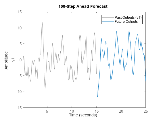
Reproduce the Output of forecast Command
This example shows how to manually reproduce forecasting results that are obtained using the forecast command. You first use the forecast command to forecast time series data into the future. You then compare the forecasted results to a manual implementation of the forecasting algorithm.
Load time series data.
load iddata9 z9
z9 is an iddata object that stores time series data (no inputs).
Specify data to use for model estimation.
observed_data = z9(1:128);
Ts = observed_data.Ts;
t = observed_data.SamplingInstants;
y = observed_data.y;
Ts is the sample time of the measured data, t is the time vector, and y is the vector of measured data.
Estimate a discrete-time state space model of 4th order.
sys = ssest(observed_data,4,'Ts',Ts);Forecast the output of the state-space model 100 steps into the future using the forecast command.
H = 100;
yh1 = forecast(sys,observed_data,H);
yh1 is the forecasted output obtained using the forecast command. Now reproduce the output by manually implementing the algorithm used by the forecast command.
Retrieve the estimated state-space matrices to create the predictor model.
A = sys.A;
K = sys.K;
C = sys.C;
Generate a 1-step ahead predictor where the A matrix of the Predictor model is A-K*C and the B matrix is K.
Predictor = idss((A-K*C),K,C,0,'Ts',Ts);Estimate initial states that minimize the difference between the observed output y and the 1-step predicted response of the identified model sys.
x0 = findstates(sys,observed_data,1);
Propagate the state vector to the end of observed data. To do so, simulate the predictor using y as input and x0 as initial states.
Input = iddata([],y,Ts);
opt = simOptions('InitialCondition',x0);
[~,~,x] = sim(Predictor,Input,opt);
xfinal = x(end,:)';
xfinal is the state vector value at time t(end), the last time instant when observed data is available. Forecasting 100 time steps into the future starts at the next time step, t1 = t(end)+Ts.
To implement the forecasting algorithm, the state vector value at time t1 is required. Compute the state vector by applying the state update equation of the Predictor model to xfinal.
x0_for_forecasting = Predictor.A*xfinal + Predictor.B*y(end);
Simulate the identified model for H steps using x0_for_forecasting as initial conditions.
opt = simOptions('InitialCondition',x0_for_forecasting);Because sys is a time series model, specify inputs for simulation as an H-by-0 signal, where H is the wanted number of simulation output samples.
Input = iddata([],zeros(H,0),Ts,'Tstart',t(end)+Ts);
yh2 = sim(sys,Input,opt);
Compare the results of the forecast command yh1 with the manually computed results yh2.
plot(yh1,yh2,'r.')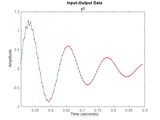
The plot shows that the results match.
Forecasting Response of Linear Models with Exogenous Inputs
When there are exogenous stimuli affecting the system, the system
cannot be considered stationary. However, if these stimuli are measurable
then you can treat them as inputs to the system and account for their
effects when forecasting the output of the system. The workflow for
forecasting data with exogenous inputs is similar to that for forecasting
time series data. You first identify a model to fit the measured input-output
data. You then specify the anticipated input values for the forecasting
time span, and forecast the output of the identified model using the forecast command.
If you do not specify the anticipated input values, they are assumed
to be zero.
This example shows how to forecast an ARMAX model with exogenous inputs in the toolbox:
Load input-output data.
load iddata1 z1
z1 is an iddata object with input-output data at 300 time points.
Use the first half of the data as past data for model identification.
past_data = z1(1:150);
Identify an ARMAX model Ay(t) = Bu(t-1) + Ce(t), of order [2 2 2 1].
na = 2; % A polynomial order
nb = 2; % B polynomial order
nc = 2; % C polynomial order
nk = 1; % input delay
sys = armax(past_data,[na nb nc nk]);
Forecast the response 100 time steps into the future, beyond the last sample of observed data past_data. Specify the anticipated inputs at the 100 future time points.
H = 100;
FutureInputs = z1.u(151:250);
forecast(sys,past_data,H,FutureInputs)
legend('Past Outputs','Future Outputs')
Forecasting Response of Nonlinear Models
The toolbox also lets you forecast data using nonlinear ARX, Hammerstein-Wiener, and nonlinear grey-box models.
Hammerstein-Wiener, and nonlinear grey-box models have a trivial
noise-component, that is disturbance in the model is described by
white noise. As a result, forecasting using the forecast command
is the same as performing a pure simulation.
Forecasting Response of Nonlinear ARX Models
A time series nonlinear ARX model has the following structure:
Where f is a nonlinear function with inputs R(t),
the model regressors. The regressors can be the time-lagged variables y(t-1), y(t-2),...
, y(t-N) and their nonlinear expressions, such
as y(t-1)2,y(t-1)y(t-2), abs(y(t-1)).
When you estimate a nonlinear ARX model from the measured data, you
specify the model regressors. You can also specify the structure of f using
different structures such as wavelet networks and tree partitions.
For more information, see the reference page for the nlarx estimation command.
Suppose that time series data from your system can be fit to a second-order linear-in-regressor model with the following polynomial regressors:
Then f(R)=W'*R+c, where W=[w1 w2 w3 w4 w5] is
a weighting vector, and c is the output offset.
The nonlinear ARX model has the form:
When you estimate the model using the nlarx command,
the software estimates the model parameters W and c.
When you use the forecast command, the
software computes the forecasted model outputs by simulating the model H time
steps into the future, using the last N measured
output samples as initial conditions. Where N is
the largest lag in the regressors, and H is the
forecast horizon you specify.
For the linear-in-regressor model, suppose that you have measured 100 samples of the output
y, and you want to forecast four steps into the future
(H = 4). The largest lag in the regressors of the model
is N = 2. Therefore, the software takes the last two samples
of the data y(99) and y(100) as initial
conditions, and forecasts the outputs as:
If your system has exogenous inputs, the nonlinear ARX model
also includes regressors that depend on the input variables. The forecasting
process is similar to that for time series data. You first identify
the model, sys, using input-output data, past_data.
When you forecast the data, the software simulates the identified
model H time steps into the future, using the last N measured
output samples as initial conditions. You also specify the anticipated
input values for the forecasting time span, FutureInputs.
The syntax for forecasting the response of nonlinear models with exogenous
inputs is the same as that for linear models, forecast(sys,past_data,H,FutureInputs).
See Also
Related Examples
- Forecast Output of Dynamic System
- Forecast Multivariate Time Series
- Time Series Prediction and Forecasting for Prognosis
More About
You can also select a web site from the following list:
Americas
- América Latina (Español)
- Canada (English)
- United States (English)
Europe
- Belgium (English)
- Denmark (English)
- Deutschland (Deutsch)
- España (Español)
- Finland (English)
- France (Français)
- Ireland (English)
- Italia (Italiano)
- Luxembourg (English)
- Netherlands (English)
- Norway (English)
- Österreich (Deutsch)
- Portugal (English)
- Sweden (English)
- Switzerland
- United Kingdom (English)