Simulate Identified Model in Simulink
After estimating a model at the command line or in the System Identification app, you can import the model from the MATLAB® workspace into Simulink® using model blocks. You can then simulate the model output for the initial conditions and the model inputs that you specify.
Add model simulation blocks to your Simulink model from the System Identification Toolbox™ block library when you want to:
Represent the dynamics of a physical component in a Simulink model using a data-based model
Replace a complex Simulink subsystem with a simpler data-based model
Summary of Simulation Blocks
The following model blocks are available in the System Identification Toolbox library in Simulink.
| Block | Description |
|---|---|
| Idmodel | Simulate a linear identified model in Simulink software. The model can be a process
(idproc), linear polynomial
(idpoly), state-space
(idss), grey-box
(idgrey), or transfer function
(idtf) model. |
| Nonlinear ARX Model | Simulate idnlarx model in Simulink. |
| Hammerstein-Wiener Model | Simulate idnlhw model in Simulink. |
| Nonlinear Grey-Box Model | Simulate nonlinear ODE (idnlgrey model
object) in Simulink. |
In any of these model blocks, you specify the model-variable name of the identified model you want to import. You also specify initial conditions for simulation (see Specifying Initial Conditions for Simulation.) You can specify time-domain input data by:
Using a From Workspace block, if one sample of input data is a scalar or vector
Using an Iddata Source block, if the input data is in an
iddataobject
For detailed information about how to configure the blocks, see the corresponding block reference pages.
Specifying Initial Conditions for Simulation
When your model is not at rest at the start of the simulation, you must specify the initial conditions. The model may not start at rest, for example, when you are:
Comparing your model response with measured output data or a previous simulation
Continuing from a previous simulation
Initiating your simulation during the steady-state phase
Initiating your simulation from a predetermined operating condition
If you do not specify initial conditions, you introduce an error source that impacts the apparent performance of your model. This error may be transient; in a model that is lightly damped or includes an integral component, the error may not completely die out.
Specifying initial conditions requires two steps:
Determine what the initial conditions should be (see Estimate Initial Conditions for Simulating Identified Models)
Specify these values as parameters in the model block.
If you have a linear model that is not idss or
idgrey, you also have to convert the model into state-space
form before the first step.
If you have already performed a simulation using compare,
sim, or the System Identification app, and you
want to check out your Simulink implementation by precisely reproducing your earlier results, see
Reproduce Command Line or System Identification App Simulation Results in Simulink.
Specifying Initial States of Linear Models
To specify initial states for state-space linear models
(idss, idgrey), use the Initial
states (state space only: idss, idgrey) parameter in the
Idmodel block. Initial states must be a vector of length equal to
the order of the model.
Other types of linear model, such as transfer-function form models
(idtf), do not use an explicit state representation. The
model blocks therefore have no input for initial state specification; the software
assumes initial conditions of zero. To specify initial conditions for one of these
models, first convert your model m into state-space form
mss at the command
line.
mss = idss(m);
mss
in the Identified model parameter of the Idmodel block. You can now specify your initial states as described in the previous
paragraph for state-space models.Simulate Identified Linear Model in Simulink with Initial Conditions
This example shows how to set the initial states for simulating a linear model such that the simulation provides a best fit to measured input-output data.
You first estimate a model M using a multiple-experiment data set Z, which contains data from three experiments - z1, z2, and z3.
Load the multi-experiment data.
load twobodiesdata
Create an iddata object to store the multi-experiment data.
z1=iddata(y1,u1,0.005);
z2=iddata(y2,u2,0.005);
z3=iddata(y3,u3,0.005);
Z = merge(z1,z2,z3);
Estimate a 5th order state-space model.
[M,x0] = n4sid(Z,5);
To simulate the model using input u2, use x0(:,2) as the initial states. x0(:,2) is computed to maximize the fit between the measured output y2 and the simulated response of M.
Extract the initial states that maximize the fit to the corresponding output y2, and simulate the model in Simulink using the second experiment, z2.
X0est = x0(:,2);
Open a preconfigured Simulink model.
mdl = 'ex_idmodel_block';
open_system(mdl)
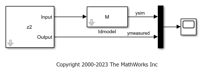
The model uses the Iddata Source, Idmodel, and Scope blocks. The following block parameters have been preconfigured to specify the simulation data, estimated model, and initial conditions.
Block parameters of Iddata Source block:
IDDATA Object -
z2Start time -
–1
Block parameters of Idmodel block:
Identified Model -
MInitial states -
X0est
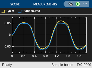
Simulate the model for two seconds, and compare the simulated output ysim with the measured output ymeasured using the Scope block.
simOut = sim(mdl);
open_system([mdl '/Scope'])
Compare this result with the result you would have gotten without setting initial conditions. You can nullify X0 in the Initial States field of the Simulink model block by replacing the X0est variable with 0. You can also nullify X0est itself in command line, as shown here.
X0est = 0*X0est;
Run the simulation, and view the new results.
simOut = sim(mdl);
open_system([mdl '/Scope'])
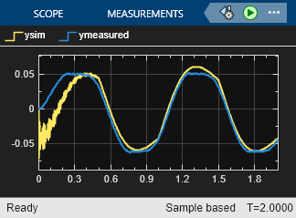
In this plot, the simulated output has a significant transient at the start, but this transient settles out in time.
Specifying Initial States of Hammerstein-Wiener Models
The states of a Hammerstein-Wiener model correspond to the states of the embedded
linear (idpoly or idss) model. For more
information about the states of a Hammerstein-Wiener model, see the idnlhw reference page.
The default initial state for simulating a Hammerstein-Wiener model is 0. For more information about specifying initial conditions for simulation, see the Hammerstein-Wiener Model reference page.
Simulate Hammerstein-Wiener Model in Simulink
Compare the simulated output of a Hammerstein-Wiener Model block to the measured output of a system. You improve the agreement between the measured and simulated responses by estimating initial state values.
Load the sample data.
load twotankdata
Create an iddata object from the sample data.
z1 = iddata(y,u,0.2,'Name','Two tank system');
Estimate a Hammerstein-Wiener model using the data.
mw1 = nlhw(z1,[1 5 3],idPiecewiseLinear,idPiecewiseLinear);
You can now simulate the output of the estimated model in Simulink using the input data in z1. To do so, open a preconfigured Simulink model.
model = 'ex_idnlhw_block';
open_system(model);

The model uses the Iddata Source, Hammerstein-Wiener Model, and Scope blocks. The following block parameters have been preconfigured to specify the estimation data, estimated model, and initial conditions:
Block parameters of Iddata Source block:
IDDATA Object -
z1Start time -
–1
Block parameters of Hammerstein-Wiener Model block:
Model -
mw1Initial conditions -
Zero(default)
Run the simulation.
View the difference between measured output and model output by using the Scope block.
simOut = sim(model);
open_system([model '/Scope'])

To improve the agreement between the measured and simulated responses, estimate an initial state vector for the model from the estimation data z1, using findstates. Specify the maximum number of iterations for estimation as 100. Specify the prediction horizon as Inf, so that the algorithm computes the initial states that minimize the simulation error.
opt = findstatesOptions;
opt.SearchOptions.MaxIterations = 100;
x0 = findstates(mw1,z1,Inf,opt);
Set the Initial conditions block parameter value of the Hammerstein-Wiener Model block to State Values. The default initial states are x0.
set_param([model '/Hammerstein-Wiener Model'],'IC','State values');
Run the simulation again, and view the difference between measured output and model output in the Scope block. The difference between the measured and simulated responses is now reduced.
simOut = sim(model);

Specifying Initial States of Nonlinear ARX Models
The states of a nonlinear ARX model correspond to the dynamic elements of the
nonlinear ARX model structure, which are the model regressors.
Regressors can be the delayed input/output variables
(standard regressors) or user-defined transformations of delayed input/output
variables (custom regressors). For more information about the states of a nonlinear
ARX model, see the idnlarx reference page.
For simulating nonlinear ARX models, you can specify the initial conditions as input/output values, or as a vector. For more information about specifying initial conditions for simulation, see the Nonlinear ARX Model reference page.
Simulate Nonlinear ARX Model in Simulink
This example shows how to compare the simulated output of a Nonlinear ARX Model block to the measured output of a system. You improve the agreement between the measured and simulated responses by estimating initial state values.
Load the sample data and create an iddata object.
load twotankdata
z = iddata(y,u,0.2,'Name','Two tank system');
z1 = z(1:1000);
Estimate a nonlinear ARX model.
mnlarx1 = nlarx(z1,[5 1 3],idWaveletNetwork(8));
You can now simulate the output of the estimated model in Simulink using the input data in z1. To do so, open a preconfigured Simulink model.
model = 'ex_idnlarx_block';
open_system(model);
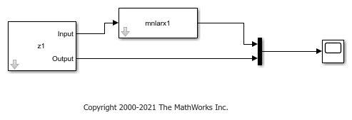
The model uses the Iddata Source, Nonlinear ARX Model, and Scope blocks. The following block parameters have been preconfigured to specify the estimation data, estimated model, and input and output levels:
Block parameters of Iddata Source block:
IDDATA Object -
z1Start time -
–1
Block parameters of Nonlinear ARX Model block:
Model -
mnlarx1Initial conditions - Input and output values (default)
Input level - 10
Output level - 0.1
Run the simulation.
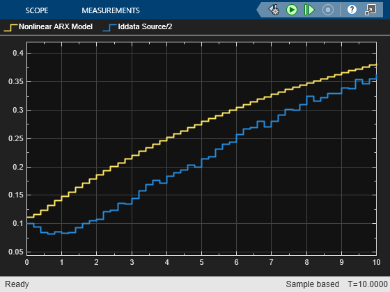
View the difference between measured output and model output by using the Scope block.
simOut = sim(model);
open_system([model '/Scope'])
To improve the agreement between the measured and simulated responses, estimate an initial state vector for the model from the estimation data, z1.
x0 = findstates(mnlarx1,z1,Inf);
Set the Initial Conditions block parameter value of the Nonlinear ARX Model block to State Values. Specify initial states as x0.
set_param([model '/Nonlinear ARX Model'],'ICspec','State values','X0','x0');
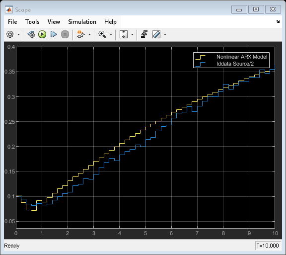
Run the simulation again, and view the difference between measured output and model output in the Scope block. The difference between the measured and simulated responses is now reduced.
simOut = sim(model);
See Also
Hammerstein-Wiener Model | Nonlinear ARX Model | Iddata Sink | Iddata Source | Idmodel
Related Topics
You can also select a web site from the following list:
Americas
- América Latina (Español)
- Canada (English)
- United States (English)
Europe
- Belgium (English)
- Denmark (English)
- Deutschland (Deutsch)
- España (Español)
- Finland (English)
- France (Français)
- Ireland (English)
- Italia (Italiano)
- Luxembourg (English)
- Netherlands (English)
- Norway (English)
- Österreich (Deutsch)
- Portugal (English)
- Sweden (English)
- Switzerland
- United Kingdom (English)