Extrapolating Scattered Data
Factors That Affect the Accuracy of Extrapolation
scatteredInterpolant provides
functionality for approximating values at points that fall outside
the convex hull. The 'linear' extrapolation method
is based on a least-squares approximation of the gradient at the boundary
of the convex hull. The values it returns for query points outside
the convex hull are based on the values and gradients at the boundary.
The quality of the solution depends on how well you’ve sampled
your data. If your data is coarsely sampled, the quality of the extrapolation
is poor.
In addition, the triangulation near the convex hull boundary can have sliver-like triangles. These triangles can compromise your extrapolation results in the same way that they can compromise interpolation results. See Interpolation Results Poor Near the Convex Hull for more information.
You should inspect your extrapolation results visually using your knowledge of the behavior outside the domain.
Compare Extrapolation of Coarsely and Finely Sampled Scattered Data
This example shows how to interpolate two different samplings of the same parabolic function. It also shows that a better distribution of sample points produces better extrapolation results.
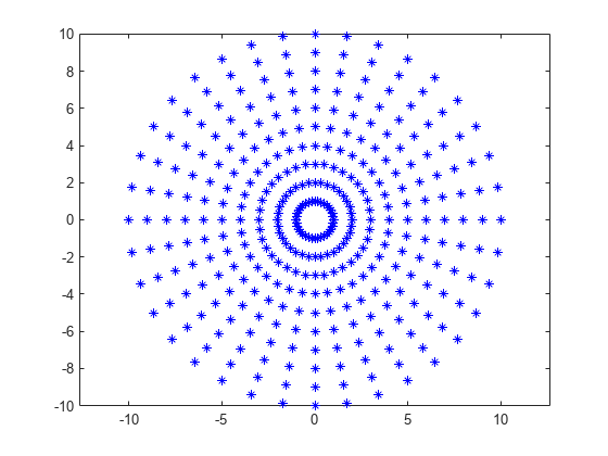
Create a radial distribution of points spaced 10 degrees apart around 10 concentric circles. Use bsxfun to compute the coordinates, and .
theta = 0:10:350;
c = cosd(theta);
s = sind(theta);
r = 1:10;

x1 = bsxfun(@times,r.',c);
y1 = bsxfun(@times,r.',s);

figure
plot(x1,y1,'*b')
axis equal
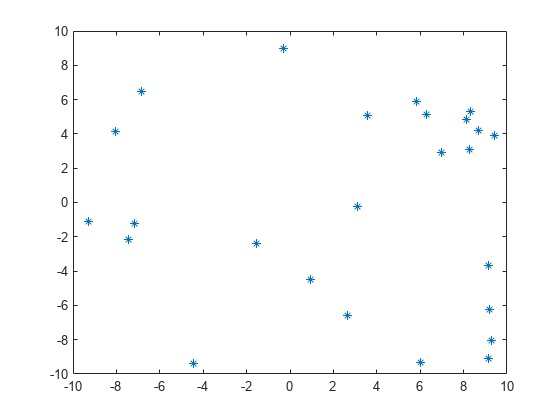
Create a second, more coarsely distributed set of points. Use the rand function to create random samplings in the range, [-10, 10].
rng default;
x2 = -10 + 20*rand([25 1]);
y2 = -10 + 20*rand([25 1]);
figure
plot(x2,y2,'*')
Sample a parabolic function, v(x,y), at both sets of points.
v1 = x1.^2 + y1.^2;
v2 = x2.^2 + y2.^2;
Create a scatteredInterpolant for each sampling of v(x,y).
F1 = scatteredInterpolant(x1(:),y1(:),v1(:));
F2 = scatteredInterpolant(x2(:),y2(:),v2(:));
Create a grid of query points that extend beyond each domain.
[xq,yq] = ndgrid(-20:20);
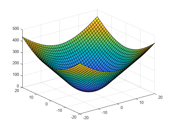
Evaluate F1 and plot the results.
figure
vq1 = F1(xq,yq);
surf(xq,yq,vq1)
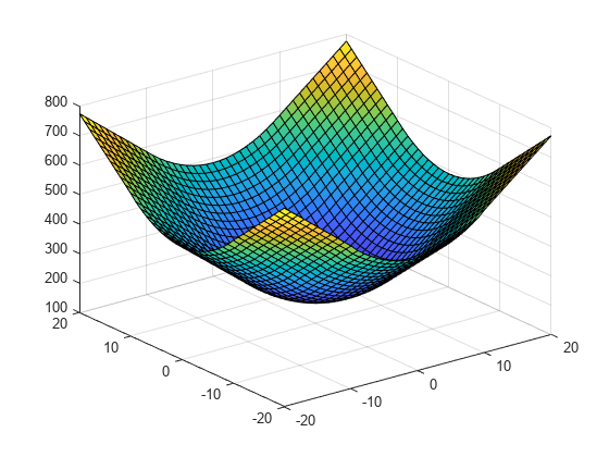
Evaluate F2 and plot the results.
figure
vq2 = F2(xq,yq);
surf(xq,yq,vq2)
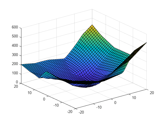
The quality of the extrapolation is not as good for F2 because of the coarse sampling of points in v2.
Extrapolation of 3-D Data
This example shows how to extrapolate a well sampled 3-D gridded dataset using scatteredInterpolant. The query points lie on a planar grid that is completely outside domain.
Create a 10-by-10-by-10 grid of sample points. The points in each dimension are in the range, [-10, 10].
[x,y,z] = ndgrid(-10:10);
Sample a function, v(x,y,z), at the sample points.
v = x.^2 + y.^2 + z.^2;
Create a scatteredInterpolant, specifying linear interpolation and extrapolation.
F = scatteredInterpolant(x(:),y(:),z(:),v(:),'linear','linear');
Evaluate the interpolant over an x-y grid spanning the range, [-20,20] at an elevation, z = 15.
[xq,yq,zq] = ndgrid(-20:20,-20:20,15);
vq = F(xq,yq,zq);
figure
surf(xq,yq,vq)
The extrapolation returned good results because the function is well sampled.