symrcm
Sparse reverse Cuthill-McKee ordering
Syntax
r = symrcm(S)
Description
r = symrcm(S) returns
the symmetric reverse Cuthill-McKee ordering of S.
This is a permutation r such that S(r,r) tends
to have its nonzero elements closer to the diagonal. This is a good
preordering for LU or Cholesky factorization of matrices that come
from long, skinny problems. The ordering works for both symmetric
and nonsymmetric S.
For a real, symmetric sparse matrix, S, the
eigenvalues of S(r,r) are the same as those of S,
but eig(S(r,r)) probably takes less time to compute
than eig(S).
Examples
The statement
B = bucky;
uses a function in the demos toolbox to generate the adjacency graph of a truncated icosahedron. This is better known as a soccer ball, a Buckminster Fuller geodesic dome (hence the name bucky), or, more recently, as a 60-atom carbon molecule. There are 60 vertices. The vertices have been ordered by numbering half of them from one hemisphere, pentagon by pentagon; then reflecting into the other hemisphere and gluing the two halves together.
With this numbering, the matrix does not have a particularly narrow bandwidth, as the first spy plot shows:
figure();
subplot(1,2,1),spy(B),title('B')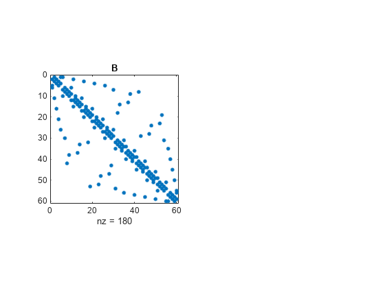
The reverse Cuthill-McKee ordering is obtained with:
p = symrcm(B);
R = B(p,p);
The spy plot shows a much narrower bandwidth.
subplot(1,2,2),spy(R),title('B(p,p)')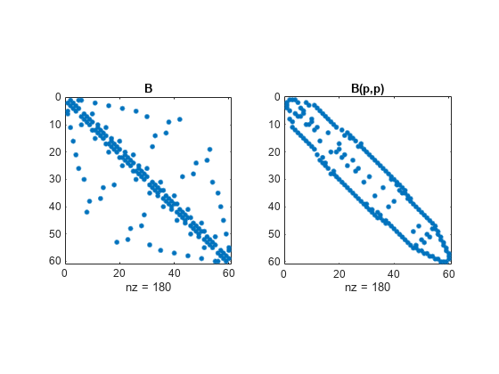
This example is continued in the reference page for symamd.
The bandwidth can also be computed with:
[i,j] = find(B);
bw = max(i-j) + 1;
The bandwidths of B and R are 35 and 12, respectively.
Algorithms
The algorithm first finds a pseudoperipheral vertex of the graph of the matrix. It then generates a level structure by breadth-first search and orders the vertices by decreasing distance from the pseudoperipheral vertex. The implementation is based closely on the SPARSPAK implementation described by George and Liu.
References
[1] George, Alan and Joseph Liu, Computer Solution of Large Sparse Positive Definite Systems, Prentice-Hall, 1981.
[2] Gilbert, John R., Cleve Moler, and Robert Schreiber, “Sparse Matrices in MATLAB: Design and Implementation,” SIAM Journal on Matrix Analysis, 1992. A slightly expanded version is also available as a technical report from the Xerox Palo Alto Research Center.
Extended Capabilities
Version History
Introduced before R2006a