Robust Control of Active Suspension
This example shows how to use Robust Control Toolbox™ to design a robust controller for an active suspension system. The example describes the quarter-car suspension model. Then, it computes an controller for the nominal system using the hinfsyn command. Finally, the example shows how to use μ-synthesis to design a robust controller for the full uncertain system.
Video Walkthrough
For a walkthrough of this example, watch the video.
Quarter-Car Suspension Model
Conventional passive suspensions use a spring and damper between the car body and wheel assembly. The spring-damper characteristics are selected to emphasize one of several conflicting objectives such as passenger comfort, road handling, and suspension deflection. Active suspensions allow the designer to balance these objectives using a feedback-controller hydraulic actuator between the chassis and wheel assembly.
This example uses a quarter-car model of the active suspension system (see Figure 1). The mass (in kilograms) represents the car chassis (body) and the mass (in kilograms) represents the wheel assembly. The spring and damper represent the passive spring and shock absorber placed between the car body and the wheel assembly. The spring models the compressibility of the pneumatic tire. The variables , , and (all in meters) are the body travel, wheel travel, and road disturbance, respectively. The force (in kiloNewtons) applied between the body and wheel assembly is controlled by feedback and represents the active component of the suspension system.
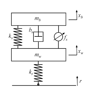
Figure 1: Quarter-car model of active suspension.
With the notation , the linearized state-space equations for the quarter-car model are:
Construct a state-space model qcar representing these equations.
% Physical parameters
mb = 300;    % kg
mw = 60;     % kg
bs = 1000;   % N/m/s
ks = 16000 ; % N/m
kt = 190000; % N/m

% State matrices
A = [ 0 1 0 0; [-ks -bs ks bs]/mb ; ...
      0 0 0 1; [ks bs -ks-kt -bs]/mw];
B = [ 0 0; 0 1e3/mb ; 0 0 ; [kt -1e3]/mw];
C = [1 0 0 0; 1 0 -1 0; A(2,:)];
D = [0 0; 0 0; B(2,:)];

qcar = ss(A,B,C,D);
qcar.StateName = ["body travel (m)";"body vel (m/s)";...
          "wheel travel (m)";"wheel vel (m/s)"];
qcar.InputName = ["r";"fs"];
qcar.OutputName = ["xb";"sd";"ab"];
The transfer function from actuator to body travel and acceleration has an imaginary-axis zero with natural frequency 56.27 rad/s. This is called the tire-hop frequency.
tzero(qcar(["xb","ab"],"fs"))
ans = 2×1 complex

  -0.0000 +56.2731i
  -0.0000 -56.2731i
Similarly, the transfer function from actuator to suspension deflection has an imaginary-axis zero with natural frequency 22.97 rad/s. This is called the rattlespace frequency.
zero(qcar("sd","fs"))
ans = 2×1 complex

  -0.0000 +22.9734i
  -0.0000 -22.9734i
Road disturbances influence the motion of the car and suspension. Passenger comfort is associated with small body acceleration. The allowable suspension travel is constrained by limits on the actuator displacement. Plot the open-loop gain from road disturbance and actuator force to body acceleration and suspension displacement.
bodemag(qcar(["ab","sd"],"r"),"b", ...
    qcar(["ab","sd"],"fs"),"r",{1 100});
legend("Road disturbance (r)","Actuator force (fs)", ...
    Location="southwest")
title(["Gain from road dist (r) and actuator force (fs)" newline ...
    "to body accel (ab) and suspension travel (sd)"])
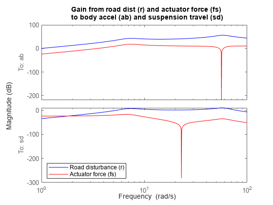
Because of the imaginary-axis zeros, feedback control cannot improve the response from road disturbance to body acceleration at the tire-hop frequency, and from to suspension deflection at the rattlespace frequency. Moreover, because of the relationship and the fact that the wheel position roughly follows at low frequency (less than 5 rad/s), there is an inherent tradeoff between passenger comfort and suspension deflection: any reduction of body travel at low frequency will result in an increase of suspension deflection.
Uncertain Actuator Model
The hydraulic actuator used for active suspension control is connected between the body mass and the wheel assembly mass . The nominal actuator dynamics are represented by the first-order transfer function with a maximum displacement of 0.05 m.
ActNom = tf(1,[1/60 1]);
This nominal model only approximates the physical actuator dynamics. We can use a family of actuator models to account for modeling errors and variability in the actuator and quarter-car models. This family consists of a nominal model with a frequency-dependent amount of uncertainty. At low frequency, below 3 rad/s, the model can vary up to 40% from its nominal value. Around 3 rad/s, the percentage variation starts to increase. The uncertainty crosses 100% at 15 rad/s and reaches 2000% at approximately 1000 rad/s. The weighting function is used to modulate the amount of uncertainty with frequency.
Wunc = makeweight(0.40,15,3);
unc = ultidyn("unc",[1 1],"SampleStateDim",5);
Act = ActNom*(1 + Wunc*unc);
Act.InputName = "u";
Act.OutputName = "fs";
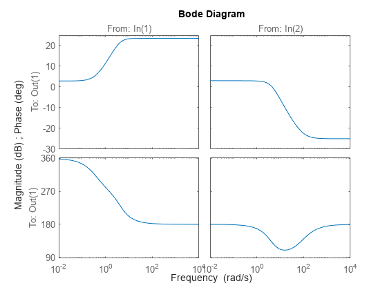
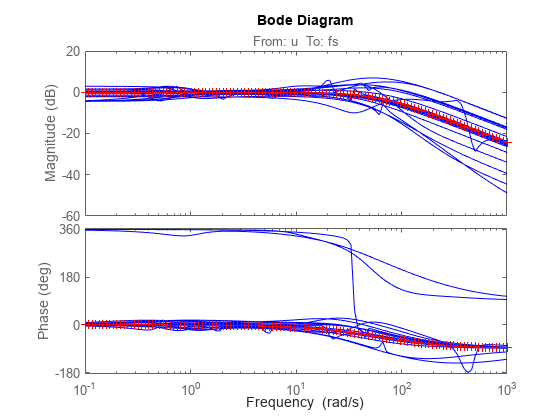
The result Act is an uncertain state-space model of the actuator. Plot the Bode response of 20 sample values of Act and compare with the nominal value.
rng("default")
bodeplot(Act,"b",Act.NominalValue,"r+",logspace(-1,3,120))
Design Setup
The main control objectives are formulated in terms of passenger comfort and road handling, which relate to body acceleration and suspension travel . Other factors that influence the control design include the characteristics of the road disturbance, the quality of the sensor measurements for feedback, and the limits on the available control force. To use synthesis algorithms, we must express these objectives as a single cost function to be minimized. This can be done as indicated Figure 2.
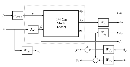
Figure 2: Disturbance rejection formulation.
The feedback controller uses measurements of the suspension travel and body acceleration to compute the control signal driving the hydraulic actuator. There are three external sources of disturbance:
The road disturbance , modeled as a normalized signal shaped by a weighting function . To model broadband road deflections of magnitude seven centimeters, we use the constant weight .
Sensor noise on both measurements, modeled as normalized signals and shaped by weighting functions and . We use and to model broadband sensor noise of intensity 0.01 and 0.5, respectively. In a more realistic design, these weights would be frequency dependent to model the noise spectrum of the displacement and acceleration sensors.
The control objectives can be reinterpreted as a disturbance rejection goal: Minimize the impact of the disturbances on a weighted combination of control effort , suspension travel , and body acceleration . When using the norm (peak gain) to measure "impact", this amounts to designing a controller that minimizes the norm from disturbance inputs to error signals .
Create the weighting functions of Figure 2 and label their I/O channels to facilitate interconnection. Use a high-pass filter for to penalize high-frequency content of the control signal and thus limit the control bandwidth.
Wroad = ss(0.07);
Wroad.u = "d1";
Wroad.y = "r";

Wact = 0.8*tf([1 50],[1 500]);
Wact.u = "u";
Wact.y = "e1";

Wd2 = ss(0.01);
Wd2.u = "d2";
Wd2.y = "Wd2";

Wd3 = ss(0.5);
Wd3.u = "d3";
Wd3.y = "Wd3";
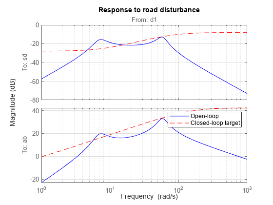
Specify closed-loop targets for the gain from road disturbance to suspension deflection (handling) and body acceleration (comfort). Because of the actuator uncertainty and imaginary-axis zeros, only seek to attenuate disturbances below 10 rad/s.
HandlingTarget = 0.04 * tf([1/8 1],[1/80 1]);
ComfortTarget = 0.4 * tf([1/0.45 1],[1/150 1]);

Targets = [HandlingTarget ; ComfortTarget];
bodemag(qcar(["sd","ab"],"r")*Wroad,"b",Targets,"r--",{1,1000})
grid
title("Response to road disturbance")
legend("Open-loop","Closed-loop target")
The corresponding performance weights are the reciprocals of these comfort and handling targets. To investigate the tradeoff between passenger comfort and road handling, construct three sets of weights corresponding to three different tradeoffs: comfort (), balanced (), and handling ().
% Three design points
beta = reshape([0.01 0.5 0.99],[1 1 3]);
Wsd = beta / HandlingTarget;
Wsd.u = "sd";
Wsd.y = "e3";
Wab = (1-beta) / ComfortTarget;
Wab.u = "ab";
Wab.y = "e2";
Finally, use connect to construct a model qcaric of the block diagram of Figure 2. Note that qcaric is an array of three models, one for each design point . Also, qcaric is an uncertain model since it contains the uncertain actuator model Act.
sdmeas  = sumblk("y1 = sd+Wd2");
abmeas = sumblk("y2 = ab+Wd3");
ICinputs = ["d1";"d2";"d3";"u"];
ICoutputs = ["e1";"e2";"e3";"y1";"y2"];
qcaric = connect(qcar(2:3,:),Act,Wroad,Wact,Wab,Wsd,Wd2,Wd3,...
                 sdmeas,abmeas,ICinputs,ICoutputs)
3x1 array of uncertain continuous-time state-space models.
Each model has 5 outputs, 4 inputs, 9 states, and the following uncertain blocks:
  unc: Uncertain 1x1 LTI, peak gain = 1, 1 occurrences
Model Properties

Type "qcaric.NominalValue" to see the nominal value and "qcaric.Uncertainty" to interact with the uncertain elements.
Nominal H-infinity Design
Use hinfsyn to compute an controller for each value of the blending factor .
ncont = 1; % one control signal, u
nmeas = 2; % two measurement signals, sd and ab
K = ss(zeros(ncont,nmeas,3));
gamma = zeros(3,1);
for i=1:3
   [K(:,:,i),~,gamma(i)] = hinfsyn(qcaric(:,:,i),nmeas,ncont);
end

gamma
gamma = 3×1

    0.9405
    0.6727
    0.8892
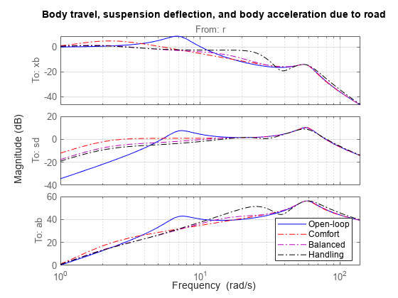
The three controllers achieve closed-loop norms of 0.94, 0.67 and 0.89, respectively. Construct the corresponding closed-loop models and compare the gains from road disturbance to for the passive and active suspensions. Observe that all three controllers reduce suspension deflection and body acceleration below the rattlespace frequency (23 rad/s).
% Closed-loop models
K.u = ["sd","ab"];
K.y = "u";
CL = connect(qcar,Act.Nominal,K,"r",["xb";"sd";"ab"]);

bodemag(qcar(:,"r"),"b", CL(:,:,1),"r-.", ...
   CL(:,:,2),"m-.", CL(:,:,3),"k-.",{1,140})
grid
legend("Open-loop","Comfort","Balanced","Handling", ...
    Location="southeast")
title(["Body travel, suspension deflection," newline ...
    "and body acceleration due to road"])
Time-Domain Evaluation
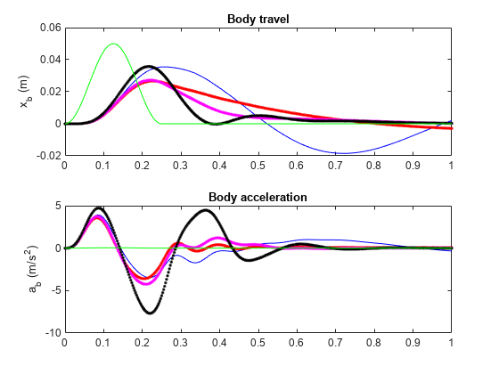
To further evaluate the three designs, perform time-domain simulations using a road disturbance signal representing a road bump of height 5 cm.
% Road disturbance
t = 0:0.0025:1;
roaddist = zeros(size(t));
roaddist(1:101) = 0.025*(1-cos(8*pi*t(1:101)));

% Closed-loop model
SIMK = connect(qcar,Act.Nominal,K,"r",["xb";"sd";"ab";"fs"]);

% Simulate
p1 = lsim(qcar(:,1),roaddist,t);
y1 = lsim(SIMK(1:4,1,1),roaddist,t);
y2 = lsim(SIMK(1:4,1,2),roaddist,t);
y3 = lsim(SIMK(1:4,1,3),roaddist,t);

% Plot results
tiledlayout(2,1);
nexttile
plot(t,p1(:,1),"b",t,y1(:,1),"r.", ...
    t,y2(:,1),"m.",t,y3(:,1),"k.", ...
    t,roaddist,"g")
title("Body travel")
ylabel("x_b (m)")
nexttile
plot(t,p1(:,3),"b",t,y1(:,3),"r.", ...
    t,y2(:,3),"m.",t,y3(:,3),"k.", ...
    t,roaddist,"g")
title("Body acceleration")
ylabel("a_b (m/s^2)")
tiledlayout(2,1);
nexttile
plot(t,p1(:,2),"b",t,y1(:,2),"r.", ...
    t,y2(:,2),"m.",t,y3(:,2),"k.", ...
    t,roaddist,"g")
title("Suspension deflection")
xlabel("Time (s)")
ylabel("s_d (m)")
nexttile
plot(t,zeros(size(t)),"b",t,y1(:,4),"r.", ...
    t,y2(:,4),"m.",t,y3(:,4),"k.", ...
    t,roaddist,"g")
title("Control force")
xlabel("Time (s)")
ylabel("f_s (kN)")
legend("Open-loop","Comfort","Balanced","Handling","Road Disturbance", ...
    Location="southeast")
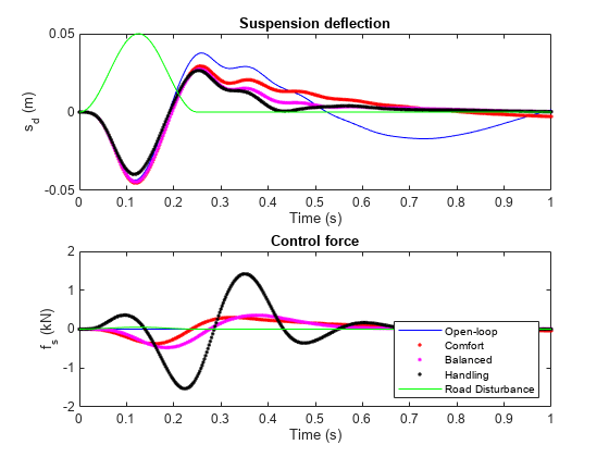
Observe that the body acceleration is smallest for the controller emphasizing passenger comfort and largest for the controller emphasizing suspension deflection. The "balanced" design achieves a good compromise between body acceleration and suspension deflection.
Robust Mu Design
So far you have designed controllers that meet the performance objectives for the nominal actuator model. As discussed earlier, this model is only an approximation of the true actuator and you need to make sure that the controller performance is maintained in the face of model errors and uncertainty. This is called robust performance.
Next use -synthesis to design a controller that achieves robust performance for the entire family of actuator models. The robust controller is synthesized with the musyn function using the uncertain model qcaric(:,:,2) corresponding to "balanced" performance ().
[Krob,rpMU] = musyn(qcaric(:,:,2),nmeas,ncont);
D-K ITERATION SUMMARY:
-----------------------------------------------------------------
                       Robust performance               Fit order
-----------------------------------------------------------------
  Iter         K Step       Peak MU       D Fit             D
    1           1.193        1.125        1.139             4
    2           1.091        1.025        1.033             4
    3          0.9991        0.946       0.9559             4
    4          0.9358        0.932       0.9348             4
    5          0.9096       0.9057       0.9114             8
    6          0.9103        0.907       0.9096             8
    7          0.9091       0.9066       0.9094             6

Best achieved robust performance: 0.906
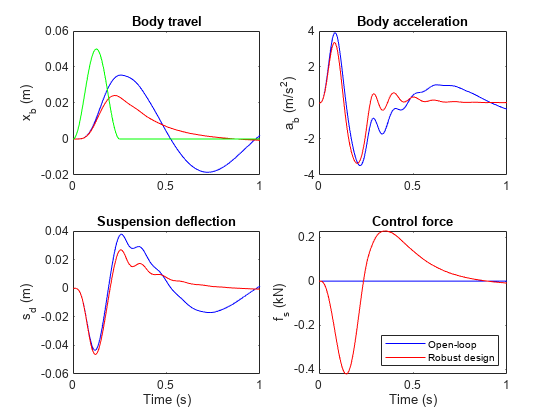
Simulate the nominal response to a road bump with the robust controller Krob. The responses are similar to those obtained with the "balanced" controller.
% Closed-loop model (nominal)
Krob.u = ["sd","ab"];
Krob.y = "u";
SIMKrob = connect(qcar,Act.Nominal,Krob,"r",["xb";"sd";"ab";"fs"]);

% Simulate
p1 = lsim(qcar(:,1),roaddist,t);
y1 = lsim(SIMKrob(1:4,1),roaddist,t);

% Plot results
clf,
tiledlayout(2,2);
nexttile
plot(t,p1(:,1),"b",t,y1(:,1),"r",t,roaddist,"g")
title("Body travel")
ylabel("x_b (m)")
nexttile
plot(t,p1(:,3),"b",t,y1(:,3),"r")
title("Body acceleration")
ylabel("a_b (m/s^2)")
nexttile
plot(t,p1(:,2),"b",t,y1(:,2),"r")
title("Suspension deflection")
xlabel("Time (s)")
ylabel("s_d (m)")
nexttile
plot(t,zeros(size(t)),"b",t,y1(:,4),"r")
title("Control force")
xlabel("Time (s)")
ylabel("f_s (kN)")
legend("Open-loop","Robust design", ...
    Location="southeast")
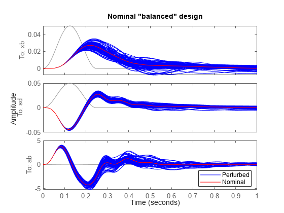
Next simulate the response to a road bump for 100 actuator models randomly selected from the uncertain model set Act.
rng("default"), nsamp = 100;  clf

% Uncertain closed-loop model with balanced H-infinity controller
CLU = connect(qcar,Act,K(:,:,2),"r",["xb","sd","ab"]);
lsimplot(usample(CLU,nsamp),"b",CLU.Nominal,"r",roaddist,t)
title("Nominal 'balanced' design")
legend("Perturbed","Nominal", ...
    Location="southeast")
% Uncertain closed-loop model with balanced robust controller
CLUrob = connect(qcar,Act,Krob,"r",["xb","sd","ab"]);
lsimplot(usample(CLUrob,nsamp),"b",CLU.Nominal,"r",roaddist,t)
title("Robust 'balanced' design")
legend("Perturbed","Nominal", ...
    Location="southeast")
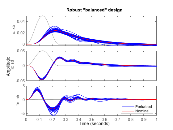
The robust controller Krob reduces variability due to model uncertainty and delivers more consistent performance.
Controller Simplification: Order Reduction
The robust controller Krob has relatively high order compared to the plant. You can use the model reduction functions to find a lower-order controller that achieves the same level of robust performance. Use reducespec and getrom to generate approximations of various orders.
% Create array of reduced-order controllers
NS = order(Krob);
StateOrders = 1:NS;
R = reducespec(Krob,"balanced");
Kred = getrom(R,Order=StateOrders,Method="truncate");
Next use robgain to compute the robust performance margin for each reduced-order approximation. The performance goals are met when the closed-loop gain is less than . The robust performance margin measures how much uncertainty can be sustained without degrading performance (exceeding ). A margin of 1 or more indicates that we can sustain 100% of the specified uncertainty.
% Compute robust performance margin for each reduced controller
gamma = 1;
CLP = lft(qcaric(:,:,2),Kred);
for k=1:NS
   PM(k) = robgain(CLP(:,:,k),gamma);
end

% Compare robust performance of reduced- and full-order controllers
PMfull = PM(end).LowerBound;
figure
plot(StateOrders,[PM.LowerBound],"b-o",...
   StateOrders,repmat(PMfull,[1 NS]),"r");
grid
title("Robust performance margin as a function of controller order")
legend("Reduced order","Full order", ...
    Location="southeast")
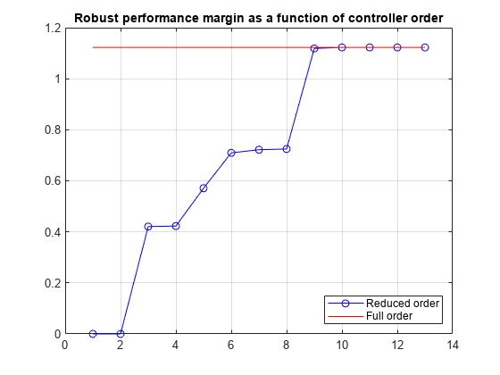
You can use the smallest controller order for which the robust performance is above 1.
Controller Simplification: Fixed-Order Tuning
Alternatively, you can use musyn to directly tune low-order controllers. This is often more effective than a-posteriori reduction of the full-order controller Krob. For example, tune a third-order controller to optimize its robust performance.
% Create tunable 3rd-order controller
K = tunableSS("K",3,ncont,nmeas);

% Tune robust performance of closed-loop system CL
CL0 = lft(qcaric(:,:,2),K);
[CL,RP] = musyn(CL0);
D-K ITERATION SUMMARY:
-----------------------------------------------------------------
                       Robust performance               Fit order
-----------------------------------------------------------------
  Iter         K Step       Peak MU       D Fit             D
    1           1.189        1.104         1.12            10
    2           1.076        1.062        1.073            10
    3          0.9905       0.9821       0.9987            10
    4          0.9268       0.9236       0.9377             6
    5          0.9251       0.9249        0.931             6
    6          0.9241       0.9236       0.9282             6

Best achieved robust performance: 0.924
The tuned controller has performance RP=0.92, very close to that of Krob. You can see its Bode response using
K3 = getBlockValue(CL,'K');
figure
bodeplot(K3)