Extract Tunable Control System from Simulink Model
This example shows how to create a tunable model for tuning with hinfstruct, starting with a Simulink® model of your control system. To do so:
Create an
slTunerinterface to the model, specifying the model elements that are tunable.Extract a linearized, tunable model from the
slTunerinterface.Define weighting functions that capture your design requirements, and incorporate them into the tunable model.
Create slTuner Interface
Open the model and create the slTuner (Simulink Control Design) interface. The interface parameterizes the tunable blocks you specify, and allows you to extract linearized open-loop and closed-loop responses from the model. For this example, use the rct_diskdrive model.
open_system('rct_diskdrive')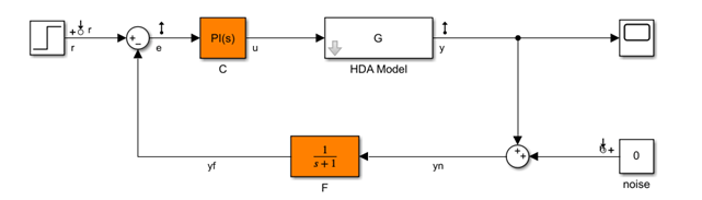
The model includes a plant model, a PI controller, and a low-pass filter in the feedback path. The model is also preconfigured with several analysis points: outputs at the error signal e and the plant output y, and additive inputs for the reference command and measurement noise. To create the slTuner interface, specify the tunable blocks.
ST0 = slTuner('rct_diskdrive',{'C','F'});
The slTuner interface automatically parametrizes these blocks using a PI controller for C and a transfer function with two free parameters for F. Because F is a low-pass filter, specify a custom parameterization to further constrain its coefficients.
a = realp('a',1);
setBlockParam(ST0,'F',tf(a,[1 a]));
Extract Tunable Closed-Loop Model
Use getIOTransfer to obtain a tunable model of the closed-loop transfer function from the reference and noise inputs {'r','n'} to the measurement and error outputs {'y','e'}.
T0 = getIOTransfer(ST0,{'r','n'},{'y','e'});
T0
Generalized continuous-time state-space model with 2 outputs, 2 inputs, 11 states, and the following blocks: C: Tunable PID controller, 1 occurrences. a: Scalar parameter, 2 occurrences. Type "ss(T0)" to see the current value and "T0.Blocks" to interact with the blocks.
This command returns a generalized LTI (genss) model with tunable blocks C and F. (For more information about tunable models, see Models with Tunable Coefficients.)
Append Weighting Functions
For hinfstruct, encode the desired response with the weighting functions that express a target loop shape LS.

Appending the transfer function LS at the error output and 1/LS at the noise input. Let T(s) denote the closed-loop transfer function from the inputs {'r','nw'} to the outputs {'y','ew'}. Then, constraining the H-infinity norm of T to less than 1 approximately enforces the target loop shape. (See Formulating Design Requirements as H-Infinity Constraints.)
For this example, use the target loop shape given by:
This value of LS corresponds to the following open-loop response shape.
wc = 1000;
s = tf('s');
LS = (1+0.001*s/wc)/(0.001+s/wc);
bodemag(LS)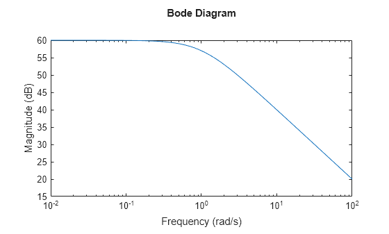
Append LS to the transfer function extracted from the slTuner interface to create the complete tunable weighted control system model.
T0 = blkdiag(1,LS) * T0 * blkdiag(1,1/LS);
You can now use hinfstruct to tune the a and the parameters in C. See Tune and Validate Controller Parameters.
See Also
Related Topics
You can also select a web site from the following list:
Americas
- América Latina (Español)
- Canada (English)
- United States (English)
Europe
- Belgium (English)
- Denmark (English)
- Deutschland (Deutsch)
- España (Español)
- Finland (English)
- France (Français)
- Ireland (English)
- Italia (Italiano)
- Luxembourg (English)
- Netherlands (English)
- Norway (English)
- Österreich (Deutsch)
- Portugal (English)
- Sweden (English)
- Switzerland
- United Kingdom (English)