Compute Open-Loop Response
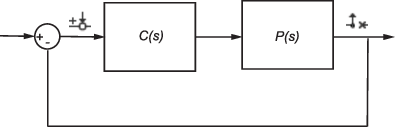
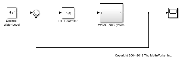
The open-loop response of a control system is the combined response of the plant and the controller, excluding the effect of the feedback loop. For example, the following block diagram shows a single-loop control system.
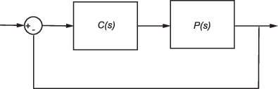
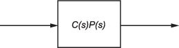
If the controller, C(s), and plant, P(s), are linear, the corresponding open-loop transfer function is C(s)P(s).
To remove the effects of the feedback loop, insert a loop opening analysis point without manually breaking the signal line. Manually removing the feedback signal from a nonlinear model changes the model operating point and produces a different linearized model. For more information, see How the Software Treats Loop Openings.
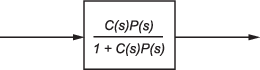
If you do not insert a loop opening, the resulting linear model includes the effects of the feedback loop.
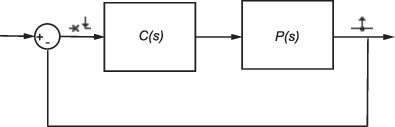
To specify the loop opening for this example, you can use either of the following analysis points.
| Analysis Point | Description | To compute C(s)P(s) |
|---|---|---|
| Specifies a loop opening followed by an input perturbation. | Specify an open-loop input at the input to the controller and an output measurement at the output of the plant.
| |
| Specifies an output measurement followed by a loop break. | Specify an open-loop output at the output of the plant and an input perturbation at the input of the controller.
|
For some systems, you cannot specify the loop opening at the same location as the
linearization input or output point. For example, to open the outer loop in the following
system, a loop opening point is added to the feedback path using a loop break analysis point
![]() . As a result, only the blue blocks are on the linearization
path.
. As a result, only the blue blocks are on the linearization
path.
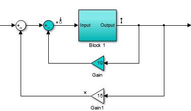
Placing the loop opening at the same location as the input or output signal would also remove the effect of the inner loop from the linearization result.
You can specify analysis points directly in your Simulink® model, in the Model Linearizer, or at the command line. For more information, about the different types of analysis points and how to define them, see Specify Portion of Model to Linearize.
Compute Open-Loop Response Using Model Linearizer
This example shows how to compute a linear model of the combined controller-plant system without the effects of the feedback signal. You can analyze the resulting linear model using, for example, a Bode plot.
Open Simulink model.
sys = 'watertank';
open_system(sys)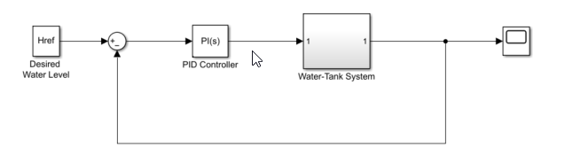
The Water-Tank System block represents the plant in this control system and contains all of the system nonlinearities.
In the Simulink model window, specify the portion of the model to linearize. For this example, specify the loop opening using open-loop output analysis point.
Open the Linearization tab. To do so, in the Apps gallery, click Linearization Manager.
To specify an analysis point for a signal, click the signal in the model. Then, on the Linearization tab, in the Insert Analysis Points gallery, select the type of analysis point.
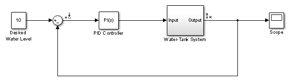
Configure the input signal of the PID Controller block as an Input Perturbation.
Configure the output signal of the Water-Tank System block as an Open-loop Output.
Annotations appear in the model indicating which signals are designated as analysis points.
Tip
If you do not want to introduce changes to the Simulink model, you can specify the analysis points in Model Linearizer. For more information, see Specify Portion of Model to Linearize in Model Linearizer.
Open Model Linearizer for the model. In the Simulink model window, in the Apps gallery, click Model Linearizer.
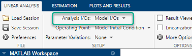
By default, the analysis points you specified in the model are selected for linearization, as displayed in the Analysis I/Os drop-down list.
To linearize the model using the specified analysis points and generate a Bode plot of
the linearized model, click ![]() Bode.
Bode.
By default, Model Linearizer linearizes the model at the model initial conditions, as shown in the Operating Point drop-down list. For examples of linearizing a model at a different operating point, see Linearize at Trimmed Operating Point and Linearize at Simulation Snapshot.
Tip
To generate response types other than a Bode plot, click the corresponding button in the plot gallery.
To view the minimum stability margins for the model, right-click the Bode plot, and select Characteristics > Minimum Stability Margins.
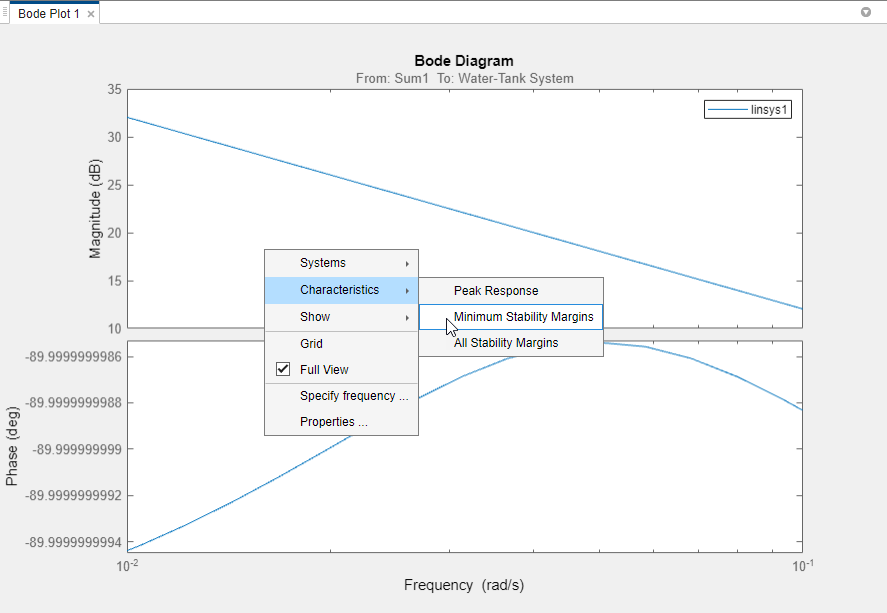
The Bode plot displays the phase margin marker. To show a data tip that contains the phase margin value, click the marker.
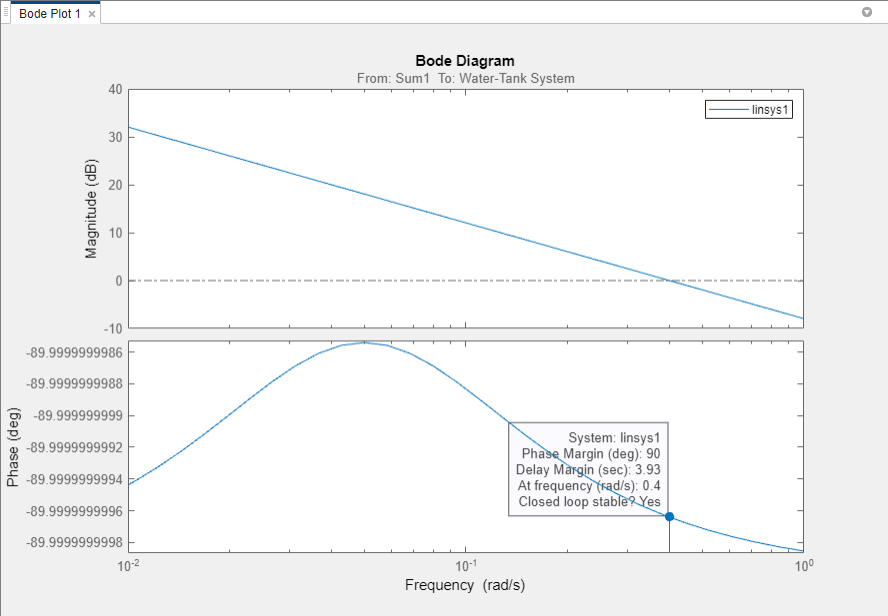
For this system, the phase margin is 90 degrees at a crossover frequency of 0.4 rad/s.
Compute Open-Loop Response at the Command Line
This example shows how to compute a linear model of the combined controller-plant system without the effects of the feedback signal. You can analyze the resulting linear model using, for example, a Bode plot.
Open Simulink model.
sys = 'watertank';
open_system(sys)
Specify the portion of the model to linearize by creating an array of analysis points using the linio command:
Open-loop input point at the input of the PID Controller block. This signal originates at the output of the Sum1 block.
Output measurement at the output of the Water-Tank System block.
io(1) = linio('watertank/Sum1',1,'openinput');
io(2) = linio('watertank/Water-Tank System',1,'output');
The open-loop input analysis point includes a loop opening, which breaks the signal flow and removes the effects of the feedback loop.
Linearize the model at the default model operating point using the linearize command.
linsys = linearize(sys,io);
linsys is the linearized open-loop transfer function of the system. You can now analyze the response by, for example, plotting its frequency response and viewing the gain and phase margins.
margin(linsys)
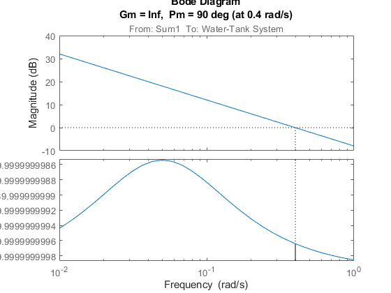
For this system, the gain margin is infinite, and the phase margin is 90 degrees at a crossover frequency of 0.4 rad/s.
See Also
Related Topics
You can also select a web site from the following list:
Americas
- América Latina (Español)
- Canada (English)
- United States (English)
Europe
- Belgium (English)
- Denmark (English)
- Deutschland (Deutsch)
- España (Español)
- Finland (English)
- France (Français)
- Ireland (English)
- Italia (Italiano)
- Luxembourg (English)
- Netherlands (English)
- Norway (English)
- Österreich (Deutsch)
- Portugal (English)
- Sweden (English)
- Switzerland
- United Kingdom (English)