Stabilize Video Using Image Point Features
This example shows how to stabilize a video that was captured from a jittery platform. One way to stabilize a video is to track a salient feature in the image and use this as an anchor point to cancel out all perturbations relative to it. This procedure, however, must be bootstrapped with knowledge of where such a salient feature lies in the first video frame. In this example, we explore a method of video stabilization that works without any such apriori knowledge. It instead automatically searches for the "background plane" in a video sequence, and uses the observed distortion to correct for camera motion.
This stabilization algorithm involves two steps. First, determine the affine image transformations between all neighboring frames of a video sequence using the estgeotform2d function applied to point correspondences between two images. Then, warp the video frames to achieve a stabilized video.
Read Frames from a Movie File
Read the first two frames of a video sequence as intensity images since color is not necessary for the stabilization algorithm, and because using grayscale images improves speed. Display both frames side by side, then create a red-cyan color composite to illustrate the pixel-wise difference between them. Note, the large vertical and horizontal offset between the two frames.
filename = "shaky_car.avi";
hVideoSrc = VideoReader(filename);

imgA = im2gray(im2single(readFrame(hVideoSrc)));
imgB = im2gray(im2single(readFrame(hVideoSrc)));

figure
tiledlayout(1,2,TileSpacing="none",Padding="tight")
nexttile
imshow(imgA)
title("Frame A")
nexttile
imshow(imgB)
title("Frame B")
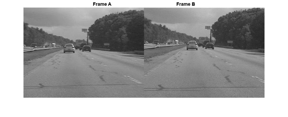
figure
imshowpair(imgA,imgB,ColorChannels="red-cyan");
title("Color composite (frame A = red,frame B = cyan)");

Collect Salient Points from Each Frame
The goal is to determine a transformation that corrects the distortion between two frames. The estgeotform2d function facilitates this by returning an affine transformation. This function requires a set of point correspondences between the two frames as input. To generate these correspondences, points of interest from both frames are first collected, followed by the selection of likely correspondences between them.
This step involves producing candidate points for each frame. To increase the likelihood of finding corresponding points in the other frame, it is advantageous to focus on points around salient image features such as corners. The detectFASTFeatures function, known for its rapid corner detection capabilities, is employed for this purpose.
ptThresh = 0.1;
pointsA = detectFASTFeatures(imgA,MinContrast=ptThresh);
pointsB = detectFASTFeatures(imgB,MinContrast=ptThresh);
The detected points from both frames are shown in the images. Observe how many of the points cover the same image features, including points along the tree line, the corners of the large road sign, and the corners of the cars.
figure
imshow(imgA)
hold on
plot(pointsA)
title("Corners in A")

figure
imshow(imgB)
hold on
plot(pointsB)
title("Corners in B")

Select Correspondences Between Points
Correspondences between the derived points are selected. For each point, a Fast Retina Keypoint (FREAK) descriptor is extracted, centered around it. The matching cost between points utilizes the Hamming distance, given that FREAK descriptors are binary. Points in frame A and frame B are putatively matched without a uniqueness constraint, allowing points from frame B to correspond to multiple points in frame A.
Extract FREAK descriptors for the corners.
[featuresA,pointsA] = extractFeatures(imgA,pointsA);
[featuresB,pointsB] = extractFeatures(imgB,pointsB);
Match features which were found in the current and the previous frames. Since the FREAK descriptors are binary, the matchFeatures function uses the Hamming distance to find the corresponding points.
indexPairs = matchFeatures(featuresA,featuresB);
pointsA = pointsA(indexPairs(:,1),:);
pointsB = pointsB(indexPairs(:,2),:);
The image displays the same color composite as given above, with the addition of points from frame A in red and points from frame B in green. Yellow lines are drawn between points to illustrate the correspondences selected by the procedure. While many of these correspondences are correct, a significant number of outliers are also present.
figure
showMatchedFeatures(imgA,imgB,pointsA,pointsB)
legend("A","B")

Estimate Transformations from Noisy Correspondences
Many point correspondences obtained in the previous step are incorrect. However, a robust estimate of the geometric transformation between the two images can still be derived using the M-estimator Sample Consensus (MSAC) algorithm, a variant of the RANSAC algorithm. The MSAC algorithm is implemented in the estgeotform2d function. This function searches for valid inlier correspondences among a set of point correspondences and uses these to derive the affine transformation. This transformation aligns the inliers from the first set of points closely with the inliers from the second set. The resulting affine transformation is represented by a 3-by-3 matrix.
[a_1 a_2 t_x;
 a_3 a_4 t_y;
  0   0    1]
The parameter define scale, rotation, and shearing effects of the transformation, and the parameter are translation parameters. This transformation can be used to warp the images such that their corresponding features will be moved to the same image location.
A limitation of the affine transformation is that it can only alter the imaging plane. Thus it is ill-suited to finding the general distortion between two frames taken of a 3-D scene, such as with this video taken from a moving car. But it does work under certain conditions that we shall describe shortly.
[tform,inlierIdx] = estgeotform2d(pointsB,pointsA,"affine");
pointsBm = pointsB(inlierIdx,:);
pointsAm = pointsA(inlierIdx,:);
imgBp = imwarp(imgB,tform,OutputView=imref2d(size(imgB)));
pointsBmp = transformPointsForward(tform,pointsBm.Location);
Display a color composite showing frame A overlaid with the reprojected frame B, along with the reprojected point correspondences. The results show the inlier correspondences nearly exactly coincident. The cores of the images are both well aligned, such that the red-cyan color composite becomes almost purely black-and-white in that region.
Note, how the inlier correspondences are all in the background of the image, not in the foreground, which itself is not aligned. This is because the background features are distant enough that they behave as if they were on an infinitely distant plane. Thus, even though the affine transformation is limited to altering only the imaging plane, here that is sufficient to align the background planes of both images. Furthermore, if we assume that the background plane has not moved or changed significantly between frames, then this transformation is actually capturing the camera motion. Therefore correcting for this will stabilize the video. This condition will hold as long as the motion of the camera between frames is small enough, or, conversely, if the video frame rate is high enough.
figure
showMatchedFeatures(imgA,imgBp,pointsAm,pointsBmp)
legend('A','B')

Transformation Approximation and Smoothing
Given a set of video frames , use the above procedure to estimate the distortion between all frames and as affine transformations, . Thus the cumulative distortion of a frame relative to the first frame will be the product of all the preceding inter-frame transformations, or
All six parameters of the affine transformation above can be used, but, for numerical simplicity and stability, re-fit the matrix as a simpler scale-rotation-translation transformation. This has only four free parameters compared to the full affine transformation's six: one scale factor, one angle, and two translations. This new transformation matrix is of the form:
[s*cos(ang)  s*sin(ang)  t_x;
 s*-sin(ang) s*cos(ang)  t_y;
     0          0          1]
This conversion procedure is demonstrated by fitting the previously obtained transformation with a scale-rotation-translation equivalent. To illustrate that the error from converting the transformation is minimal, frame B is reprojected with both transformations, and the two images are displayed below as a red-cyan color composite. The near black and white appearance of the image clearly indicates that the pixel-wise difference between the different reprojections is negligible.
Extract scale and rotation part sub-matrix.
tformAffine = tform.A;
R = tformAffine(1:2,1:2);
Compute theta from mean of two possible arctangents.
theta = mean([atan2(-R(3),R(1)) atan2(R(2),R(4))]);
Compute scale from mean of two stable mean calculations.
scale = mean(R([1 4])/cos(theta));
Convert theta to degrees.
thetad = rad2deg(theta);
Translation remains the same.
translation = tformAffine(1:2,3);
Reconstitute new s-R-t transformation and store it in a simtform2d object.
tformSRT = simtform2d(scale,thetad,translation);

imgBold = imwarp(imgB,tform,OutputView=imref2d(size(imgB)));
imgBsRt = imwarp(imgB,tformSRT,OutputView=imref2d(size(imgB)));

figure(2)
clf
imshowpair(imgBold,imgBsRt,"ColorChannels","red-cyan"),axis image;
title("Color composite of affine and similarity outputs");

Run on the Full Video
Apply the above steps to smooth a video sequence. For readability, the above procedure of estimating the transformation between two images has been placed in the MATLAB® function cvexEstStabilizationTform. The function cvexTformToSRT also converts a general affine transformation into a similarity (scale-rotation-translation) transformation.
At each step, the transformation between the current frames is calculated and fitted as an s-R-t transform. This is then combined into the cumulative transformation, which describes all camera motion since the first frame. The last two frames of the smoothed video are displayed in a Video Player as a red-cyan composite. Removing the early exit condition from the code allows for processing the entire video.
Reset the video source to the beginning of the file and create a video player.
read(hVideoSrc,1);
hVPlayer = vision.VideoPlayer;
Process all frames in the video.
movMean = im2gray(im2single(readFrame(hVideoSrc)));
imgB = movMean;
imgBp = imgB;
correctedMean = imgBp;
ii = 2;
cumulativeTform = simtform2d;
For each new frame, estimate the transformation from frame A to frame B, and fit it as an s-R-t transformation. Display as a color composite with previous corrected frame. The release object function closes any open files and releases memory.
while hasFrame(hVideoSrc) && ii < 10

    imgA = imgB;
    imgAp = imgBp;
    imgB = im2gray(im2single(readFrame(hVideoSrc)));
    movMean = movMean + imgB;

    tformAffine = cvexEstStabilizationTform(imgA,imgB);
    sRtTform = cvexTformToSRT(tformAffine);
    cumulativeTform = simtform2d(cumulativeTform.A * sRtTform.A);
    imgBp = imwarp(imgB,cumulativeTform,OutputView=imref2d(size(imgB)));

    step(hVPlayer,imfuse(imgAp,imgBp,ColorChannels="red-cyan"));
    correctedMean = correctedMean + imgBp;

    ii = ii+1;
end
correctedMean = correctedMean/(ii-2);
movMean = movMean/(ii-2);

release(hVPlayer);

During computation, the process involved calculating the mean of the raw video frames and the corrected frames. The display shows these mean values side-by-side. The left image reveals the mean of the raw input frames, highlighting the significant distortion present in the original video. In contrast, the right image displays the mean of the corrected frames, showing the image core with minimal distortion. While the car's forward motion has blurred foreground details, this demonstrates the stabilization algorithm's effectiveness.
figure
tiledlayout(1,2,TileSpacing="none",Padding="tight")
nexttile
imshow(movMean)
title("Raw input mean")
nexttile
imshow(correctedMean)
title("Corrected sequence mean")

References
[1] Tordoff, B; Murray, DW. "Guided sampling and consensus for motion estimation." European Conference n Computer Vision, 2002.
[2] Lee, KY; Chuang, YY; Chen, BY; Ouhyoung, M. "Video Stabilization using Robust Feature Trajectories." National Taiwan University, 2009.
[3] Litvin, A; Konrad, J; Karl, WC. "Probabilistic video stabilization using Kalman filtering and mosaicking." IS&T/SPIE Symposium on Electronic Imaging, Image and Video Communications and Proc., 2003.
[4] Matsushita, Y; Ofek, E; Tang, X; Shum, HY. "Full-frame Video Stabilization." Microsoft® Research Asia. CVPR 2005.