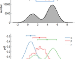
%% description
% function [theText, rawN, x] = nhist(cellValues, 'parameter', value, ...)
%
% nhist(x); works just like hist(x) but the resulting plot looks nice.
%
% t = nhist(Y) bins the elements of Y into equally spaced containers
% and returns a string with information about the distributions.
% If Y is a cell array or a structure nhist will make graph the
% binned (discrete) probability density function of each data
% set for comparison on the same graph. It will return A cell
% array or structure which includes a string for each set of
% data.
%
% [t, N, X]= nhist(...) also returns the number of items in each bin, N,
% and the locations of the left edges of each bin. If Y is a
% cell array or structure then the output is in the same form.
%
% nhist(Y,'PropertyName', . . . )
% nhist(Y,'PropertyName',PropertyValue, . . . )
% See below for the different parameters.
%__________________________________________________________________________
% Summary of what function does:
% 1) Automatically sets the number and range of the bins to be appropriate
% for the data.
% 2) Compares multiple sets of data elegantly on one or more plots, with
% legend or titles. It also graphs the mean and standard deviations.
% It can also plot the median and mode.
% 3) Outputs text with the usefull statistics for each distribution.
% 4) Allows for changing many more parameters
%
% Highlighted features (see below for details)
% 'separate' to plot each set on its own axis, but with the same bounds
% 'binfactor' change the number of bins used, larger value =more bins
% 'samebins' force all bins to be the same for all plots
% 'legend' add a legend in the graph (default for structs)
% 'noerror' remove the mean and std plot from the graph
% 'median' add the median of the data to the graph
% 'text' return many details about each graph even if not plotted
% The function is robust to NaN and +-inf data points (with warnings)
%
%% Optional Properties
% Note: Alternative names to call the properties are listed at the end of each
% entry.
%__________________________________________________________________________
% Histogram and bin settings
% 'binfactor': Effects the number of bins used. A larger number
% will mean more bins used. All bins will be some
% multiple of the largest bin.
% 'binfactor','binfactors','factor','f'
% 'samebins': this will make all the bins align with each other
% the binwidth will be the mean of all the
% recomended bin sizes.
% 'minbins': The minimum number of bins allowed for each graph
% default = 10. 'minimumbins'
% 'maxbins': The maximum number of bins allowed for each graph
% default = 100. 'maximumbins'
% 'stdtimes': Number of times the standard deviation to set the
% horizontal limits of the axis, default is 4.
% 'minx': crop the axis and histogram on the left. 'xmin'
% 'maxx': crop the axis and histogram on the right. 'xmax'
% 'proportion': Plot proportion of total points on the y axis
% rather than the totaly number of points or the
% probability distribution. Useful for data sets
% with small sample sizes. 'p'
% 'pdf': Plot the pdf on the y axis
% 'numbers': Plot the raw numbers on the graph. 'number'
% 'smooth': Plot a smooth line instead of the step function.
% 'int': Force it to make bins along integers. If you like
% pass 1 or 0 to force int bins, or relax the
% restriction if it is imposed automatically.
% 'integer','discrete','intbins'
%__________________________________________________________________________
% Text related parameters
% 'titles','legend': A cell array with strings to put in the legend or
% titles. Also used for text output. 'title'
% 'nolengend': In case you pass a struct, you may force a legend
% to disappear. You will have no way to track the
% data.
% 'text': Outputs all numbers to text, even ones that are
% not plotted, this will include the number of
% points, mean, standard deviation, standard error,
% median, and approximate mode., 't','alltext'
% 'decimalplaces': Number of decimal places numbers will be output
% with, 'decimal', 'precision', 'textprecision'
% 'npoints': this will add (number of points) to the legend or
% title automatically for each plot. 'points'
% 'xlabel': Label of the lowest X axis
% 'ylabel': Label of the Y axis, note that the ylabel default
% will depend on the type of plot used, it will vary
% from 'pdf' (or probability distribution) for
% regular plots, 'number' for separate plots (the
% number of elements) and 'proportion' for
% proportion plots. Setting this parameter will
% override the defaults.
% 'fsize': Font size, default 12. 'fontsize'
% 'location': Sets the location of the legend,
% example:NorthOutside. 'legendlocation'
%__________________________________________________________________________
% Peripheral elements settings
% 'median': This will plot a stem plot of the median
% 'mode': This will plot a stem plot of the mode
% If both 'mode' and 'median' are passed, the mode
% will be plotted with a dashed line.
% 'serror': Will put the mean and 'standard error' bars above
% the plot rather than the default standard
% deviation. 'serrors','stderror','stderrors','sem'
%
% 'noerror': Will remove the mean and standard deviation error
% bars from above the plot. 'noerrors,
% 'linewidth': Sets the width of the lines for all the graphs
% 'color': Sets the colors of the lines.
% 'qualitative' forces each line to be most
% distinguishable, up to 12 different colors.
% 'sequential' forces the colors into a smooth
% spectrum from red to blue.
% 'colormap' will take the colors from the existing
% colormap, allowing you to choose them freely.
% 'jet' setting the parameter to an regular colormap
% will choose the colors from that map
% 'jet','gray','summer','cool', etc.
% For 'separate' plots color will specify the color of the
% bar graphs. You must use the [R G B] standard
% color definitions.
%__________________________________________________________________________
% General Figure Settings
% 'separate': Plot each histogram separately, also use normal
% bar plots for the histograms rather than the
% stairs function. Data will not be normalized.
% 'separateplots','plotseparately','normalhist','normal','s'
% 'newfig': Will make a new figure to plot it in. When using
% 'separateplots' 'newfig' will automatically
% change the size of the figure.
% 'eps': EPS file name of the generated plot to save. It
% will automatically print if you pass this
% parameter
%
%% The bin width is defined in the following way
% Disclaimer: this function is specialized to compare data with comparable
% standard deviations and means, but greatly varying numbers of points.
%
% Scotts Choice used for this function is a theoretically ideal way of
% choosing the number of bins. Of course the theory is general and so not
% rigorous, but I feel it does a good job.
% (bin width) = 3.5*std(data points)/(number of points)^(1/3);
%
% I did not follow it exactly though, restricting smaller bin sizes to be
% divisible by the larger bin sizes. In this way the different conditions
% can be accurately compared to each other.
%
% The bin width is further adulterated by user parameter 'binFactor'
% (new bin width) = (old bin width) / (binFactor);
% it allows the user to make the bins larger or smaller to their tastes.
% Larger binFactor means more bins. 1 is the default
%
%Source: http://en.wikipedia.org/wiki/Histogram#Number_of_bins_and_width
%
%% Default function behaviour
%
% If you pass it a structure, the field names will become the legend. All
% of the data outputted will be in structure form with the same field
% names. If you pass a cell array, then the output will be in cell form. If
% you pass an array or vector then the data is outputted as a string and
% two arrays.
%
% standard deviation will be plotted as a default, unless one puts in the
% 'serror' paramter which will plot the standard error = std/sqrt(N)
%
% There is no maximum or minimum X values.
% minBins=10; The minimum number of bins for the histogram
% maxBins=100;The maximum number of bins for a histogram
% AxisFontSize = 12; 'fsize' the fontsize of everything.
% The number of data points is not displayed
% The lines in the histograms are black
% faceColor = [.7 .7 .7]; The face of the histogram is gray.
% It will plot inside a figure, unless 'newfig' is passed then it will make
% a new figure. It will take over and refit all axes.
% linewidth=2; The width of the lines in the errobars and the histogram
% stdTimes=4; The axes will be cutoff at a maximum of 4 times the standard
% deviation from the mean.
% Different data sets will be plotted with a different number of bins.
%% Acknowledgments
% Thank you to the AP-Lab at Boston University for funding me while I
% developed this function. Thank you to the AP-Lab, Avi and Eli for help
% with designing and testing it and the Mathworks community for comments!
%% Examples
% Cell array example:
% A={randn(1,10^5),randn(10^3,1)+1};
% nhist(A,'legend',{'\mu=0','\mu=1'});
% nhist(A,'legend',{'\mu=0','\mu=1'},'separate');
%
% A=[randn(1,10^5)+1 randn(1,2*10^5)+5];
% nhist(A,'mode')
%
% Structure example:
% A.mu_is_Zero=randn(1,10^5); A.mu_is_Two=randn(10^3,1)+2;
% nhist(A);
% nhist(A,'color','summer')
% nhist(A,'color',[.3 .8 .3],'separate')
% nhist(A,'binfactor',4)
% nhist(A,'samebins')
% nhist(A,'median','noerror')
%%%%%%%%%%%%%%%%%%%%%%%%%%%%%%%%%%%%%%%%%%%%%%%%%%%%%%%%%%%%%%%%%%%%%%%%%%%
% Jonathan Lansey 2010-2013, %
% questions to Lansey at gmail.com %
%%%%%%%%%%%%%%%%%%%%%%%%%%%%%%%%%%%%%%%%%%%%%%%%%%%%%%%%%%%%%%%%%%%%%%%%%%%
function [theText,rawN, x] = nhist(cellValues, varargin)
%% INITIALIZE PARAMETERS
% Default initialization of the parameters,
stdTimes=4; % the number of times the standard deviation to set the upper end of the axis to be.
binFactor=1.5;
sameBinsFlag=0; % if 1 then all bins will be the same size
proportionFlag=0;
pdfFlag = 0;
numberFlag = 0;
smoothFlag = 0;
intbinsForcedFlag = 0;
intbinsFlag = 0;
% These are used later to set the output parameters right.
structFlag=0;
arrayFlag=0;
minX=[]; % for the axis in case users don't enter anything
maxX=[];
minBins=10;
maxBins=100;
SXLabel = '';
yLabelFlag=0;
EPSFileName = '';
Title = '';
AxisFontSize = 12;
npointsFlag=0;
legendLocation='best';
forceNoLegend=0;
% lineColor = [.49 .49 .49];
lineColor = [0 0 0];
faceColor = [.7 .7 .7];
vertLinesForcedFlag=0;
multicolorFlag=0;
brightnessExponent=1/2;
plotStdFlag = 1; % 1 if either serror or std will be plotted
serrorFlag = 0;
medianFlag = 0;
modeFlag = 0;
boxplotFlag = 0;
textFlag=0;
decimalPlaces=2;
legendExists=0;
linewidth=2;
newfigFlag=0;
barFactor=1;
normalHist=0;
%% Interpret the user parameters
k = 1;
while k <= length(varargin)
if ischar(varargin{k})
switch (lower(varargin{k}))
case {'legend','titles','title'}
cellLegend=varargin{k+1};
legendExists=1;
k = k + 1;
case {'location','legendlocation'}
legendLocation=varargin{k+1};
k = k + 1;
case 'nolegend'
forceNoLegend=1;
case 'xlabel'
SXLabel = varargin{k + 1};
k = k + 1;
case 'ylabel'
SYLabel = varargin{k + 1};
yLabelFlag=1;
k = k + 1;
case {'minx','xmin'}
minX = varargin{k + 1};
k = k + 1;
case {'maxx','xmax'}
maxX = varargin{k + 1};
k = k + 1;
case {'minbins','minimumbins'}
minBins = varargin{k + 1};
k = k + 1;
case {'maxbins','maximumbins'}
maxBins = varargin{k + 1};
k = k + 1;
case 'stdtimes' % the number of times the standard deviation to set the upper end of the axis to be.
stdTimes = varargin{k + 1};
k = k + 1;
if ischar(stdTimes)
fprintf(['\nstdTimes set to: ' stdTimes]);
error('stdTimes must be a number')
end
case {'binfactor','binfactors','factor','f'}
binFactor = varargin{k + 1};
k = k + 1;
if ischar(binFactor)
error('binFactor must be a number')
end
case {'samebins','samebin','same'}
sameBinsFlag=1;
case {'proportion','p'}
proportionFlag=1;
case 'pdf'
pdfFlag=1;
case {'numbers','number'}
numberFlag = 1;
case 'smooth'
smoothFlag = 1;
case {'int','integer','discrete','intbins','intbin'}
intbinsForcedFlag = 1;
intbinsFlag=1;
if k+1<= length(varargin)
temp = varargin{k + 1};
if ~ischar(temp) % if its a number then we want to use it.
intbinsFlag=temp;
end
end
case 'eps'
EPSFileName = varargin{k + 1};
k = k + 1;
case {'fsize','fontsize'}
AxisFontSize = varargin{k + 1};
k = k + 1;
case 'linewidth'
linewidth = varargin{k + 1};
k = k + 1;
case {'color','colors'}
lineColor=varargin{k+1};
if ischar(lineColor)
% if strcmp(lineColor,'multicolor')
multicolorFlag = 1;
% end
else %then lineColor will be redone later
faceColor = lineColor;
end
k = k + 1;
case {'npoints','points'}
npointsFlag=1;
case {'lines','line'}
vertLinesFlag=1;
vertLinesForcedFlag=vertLinesForcedFlag+1;
case {'noline','nolines'}
vertLinesFlag=0;
vertLinesForcedFlag=vertLinesForcedFlag+1;
case { 'decimalplaces','decimal','precision','textprecision'}
decimalPlaces=varargin{k+1};
k=k+1;
case {'newfig','newfigure'}
newfigFlag=true;
case {'noerror','noerrors'}
plotStdFlag = 0;
case {'serror','serrors','stderror','stderrors','sem'}
serrorFlag = 1;
case {'boxplot','bplot','box'} % surprise! undocumented feature.
boxplotFlag = 1;
plotStdFlag = 0;
case {'barwidth','barfactor','errorbarwidth'}
barFactor = varargin{k+1};
k = k+1;
case {'median','medians'}
medianFlag=1;
case {'separateplots','separate','plotseparately','normalhist','normal','s'}
normalHist=1;
case {'mode','modes'}
modeFlag = 1;
case {'text','alltext','t'}
textFlag=1;
otherwise
warning('user entered parameter is not recognized')
disp('unrecognized term is:'); disp(varargin{k});
end
end
k = k + 1;
end
% intbinsForcedFlag
% intbinsFlag
%% Check if data is an array, not a cell
valueInfo=whos('cellValues');
valueType=valueInfo.class;
switch valueType
case 'cell' % There are a few cells there, it will run as usual.
% normalHist=what you set it to, or zero;
case 'struct'
structFlag=1;
tempValues=cellValues; clear('cellValues');
if legendExists
warning(['The legend you entered will be ignored and replaced '...
'with field names. Use a cell array to pass your own legend, '...
'or rename the fields']);
else % set it to Exists,
if forceNoLegend
legendExists=0;
else
legendExists=1;
end
end
forStructLegend=fields(tempValues)';
for k=1:length(forStructLegend)
cellValues{k}=tempValues.(forStructLegend{k});
end
cellLegend =forStructLegend; % this is for text purposes.
otherwise % Its an array and data needs to be changed to a cell array, for what follows.
arrayFlag=1;
cellValues={cellValues};
normalHist=1;
if legendExists % it is probably passed as a string not a cell
valueInfo=whos('cellLegend');
valueType=valueInfo.class;
if ~strcmp(valueType,'cell')
cellLegend={cellLegend};
else
warning('please pass the legend as the same type as the data');
end
end
end
%% Check some user-entered parameters for problems
if round(decimalPlaces)~=decimalPlaces
warning(['decimalPlaces must be an integer number. You entered ' num2str(decimalPlaces) ' '...
'the rounded number ' num2str(round(decimalPlaces)) ' will be used instead']);
decimalPlaces=round(decimalPlaces);
end
if vertLinesForcedFlag>1
warning(['you cannot specify having and not having vertical lines. ' ...
'Therefore we will determine it automatically as usual']);
vertLinesForcedFlag=0;
end
%% Collect the Data, check some things
num2Plot=length(cellValues);
if legendExists
if num2Plot~=length(cellLegend)
warning('legend is not appropriately sized for the data');
if num2Plot>length(cellLegend)
for k=length(cellLegend)+1:num2Plot
cellLegend{k}=['Plot #' num2str(k)];
end
end
end
end
% check for integer, or near integer values (to make integer bins without gaps)
if intbinsFlag
intbins=ones(1,num2Plot);
else
intbins=zeros(1,num2Plot);
if ~intbinsForcedFlag % if its forced, then we want it to stay zero
for k=1:num2Plot
intbins(k) = isdiscrete(cellValues{k});
end
if sameBinsFlag % then if one has integers, they all must be plotted along integers.
intbins = or(intbins,sum(intbins));
end
end
end
% This is to collect the means std, and a few other things
for k=1:num2Plot
if ~isnumeric(cellValues{k})
error(['You cannot make a histogram of non-numeric data. Plot #' num2str(k) ' non numeric']);
end
% infFlag(k)=;
% Changing numbers to doubles makes the 'text' parameter work.
% This also makes it so you can pass it a full matrix, just for fun.
% It is done for each one individually so you can even pass a cell array
% where the individual vectors are differently angled.
cellValues{k}=double(cellValues{k}(:));
nanValues = isnan(cellValues{k});
nnan = sum(nanValues);
% remove NaN values
if nnan>0
cellValues{k}=cellValues{k}(~nanValues);
if nnan>1, waswere='were'; else waswere='was';end
warning(['data set #:' num2str(k) ' has ' num2str(nnan) ' ''NaN'' values which ' waswere ' removed from all analysis and counts\n']);
end
% Check for and deal with infinite values.
infValues=isinf(cellValues{k});
if sum(infValues)%infFlag(k)
plotStdFlag=0; % the mean of the data makes no sense here.
if sum(infValues)>1, waswere='were'; else waswere='was';end
warning(['data set #:' num2str(k) ' has ''inf'' values which ' waswere ' put in the end bin/s. The mean and std will not be displayed\n']);
infV=cellValues{k}(infValues);
nPosInf=sum(infV>0);
nNegInf=sum(infV<0);
cellValues{k}=cellValues{k}(~infValues);
else
nPosInf=0;
nNegInf=0;
end
% Store the values temporarily
Values=cellValues{k};
% check for imaginary data
if ~isreal(Values)
warning('magnitude taken of all imaginary data');
Values=abs(Values);
cellValues{k}=Values;
end
% check if it is an empty bin
if isempty(Values)
isData(k)=false;
Values=[0 0 0];
cellValues{k}=Values;
warning(['data set #:' num2str(k) ' is empty']);
else
isData(k)=true;
end
% Store a few other useful values
stdV{k}=std(Values); % standard dev of values
meanV{k}=mean(Values);
medianV{k}=median(Values);
numPoints{k}=length(Values); % number of values
% initialize to be used later, not a user paramter at all
modeShift{k}=0;
end
if sum(isData)<1
warning('None of your data is plottable, so nothing was plotted. Please search for more data and try again');
return;
end
%% FIND THE AXIS BOUNDS
% on each side, left and right
% error the user if they choose retarded bounds (pardon my politically uncorrectness)
if ~isempty(minX) && ~isempty(maxX)
if maxX<minX
error(['your max bound: ' num2str(maxX) ' is bigger than your min bound: ' num2str(minX) ' you can''t do that silly']);
end
end
for k=1:num2Plot
Values=cellValues{k};
% warn error if there is only one point of data
if length(Values)<2
warning(['maybe a histogram is not the best method to graph your single number in plot#:' num2str(k)]);
end
% warn the user if they chose a dumb bounds (but not retarded ones)
if ~isempty(minX)
if minX>meanV{k}
warning(['the mean of your data set#' num2str(k) ' is off the chart to the left, '...
'choose larger bounds or quit messing with the program and let it do '...
'its job the way it was designed.']);
end
end
if ~isempty(maxX)
if maxX<meanV{k}
warning(['the mean of your data set#' num2str(k) ' is off the chart to the right, '...
'choose larger bounds or quit messing with the program and let it do '...
'its job the way it was designed.']);
end
end
% Note the check stdV{k}>0, just in case the std is zero, we need to set
% boundaries so that it doesn't crash with 0 bins used. The range of
% (+1,-1) is totally arbitrary.
% set x MIN values
if isempty(minX) % user did not specify - then we need to find the minimum x value to use
if stdV{k}>0 % just checking there are more than two different points to the data
leftEdge = meanV{k}-stdV{k}*stdTimes;
if leftEdge<min(Values) % if the std is larger than the largest value
minS(k)=min(Values);
else % cropp it now on the bottom.
% cropped!
minS(k) = leftEdge;
end
else % stdV==0, wow,
minS(k)=min(Values)-eps;
end
else % minX is specified so minS is just set stupidly here
minS(k)=minX;
end
% set x MAX values
if isempty(maxX)
if stdV{k}>0 % just checking there are more than two different points to the data
rightEdge = meanV{k}+stdV{k}*stdTimes;
if rightEdge>max(Values) % if the suggested border is larger than the largest value
maxS(k)=max(Values);
else % crop the graph to cutoff values
maxS(k)=rightEdge;
end
else % stdV==0, wow,
% Note that minX no longer works in this case.
maxS(k)=max(Values)+eps;
end
else % maxX is specified so minS is just set here
maxS(k)=maxX;
end
if intbins(k)
maxS(k)=round(maxS(k))+.5;
minS(k)=round(minS(k))-.5; % subtract 1/2 to make the bin peaks appear on the numbers.
end
end % look over k finished
% This is the range that the x axis will plot at for each one.
% Only set the bounds for things that have data
% isData = logical(isData);
SXRange = [min(minS(isData)) max(maxS(isData))];
% note that later there will be a bit added to maxS of SXRange
% This below is to get estimates for appropriate binsizes
totalRange=diff(SXRange);
%% deal with the infinity data
% In this case we add the inf values back in as off the charts numbers on
% the appropriate side. In this way the 'cropped' star will be plotted.
for k=1:num2Plot % nNegInf= number of negative infinities removed
cellValues{k}=[cellValues{k}; repmat(SXRange(1)-100,nNegInf,1); repmat(SXRange(2)+100,nPosInf,1)];
end
%% FIND OUT IF THERE WERE CROPS DONE
for k=1:num2Plot
% Set the crop flag
if min(cellValues{k})<SXRange(1)
cropped_left{k}=sum(cellValues{k}<SXRange(1)); % flag to plot the star later
else
cropped_left{k}=0;
end
% Set the crop flag
if max(cellValues{k})>SXRange(2)
cropped_right{k}=sum(cellValues{k}>SXRange(2)); % flag to plot the star later
else
cropped_right{k}=0;
end
end
%% DEAL WITH BIN SIZES
% Reccomend a bin width
binWidth=zeros(1,num2Plot);
% Warn users for dumb max/min bin size choices.
if minBins<3, error('No I refuse to plot this you abuser of functions, the minimum number of bins must be at least 3'); end;
if minBins<10, warning('you are using a very small minimum number of bins, do you even know what a histogram is?'); end;
if minBins>20, warning('you are using a very large minimum number of bins, are you sure you *always need this much precision?'); end;
if maxBins>150,warning('you are using a very high maximum for the number of bins, unless your monitor is in times square you probably won''t need that many bins'); end;
if maxBins<50, warning('you are using a low maximum for the number of bins, are you sure it makes sense to do this?'); end;
% Choose estimate bin widths
for k=1:num2Plot
% This formula "Scott's choice" is described in the introduction above.
% default: binFactor=1;
binWidth(k)=3.5*stdV{k}/(binFactor*(numPoints{k})^(1/3));
% Instate a mininum and maximum number of bins
numBins = totalRange/binWidth(k); % Approx number of bins
if numBins<minBins % if this will imply less than 10 bins
binWidth(k)=totalRange/(minBins); % set so there are ten bins
end
if numBins>maxBins % if there would be more than 75 bins (way too many)
binWidth(k)=totalRange/maxBins;
end
% Check if it is intbins, becase then:
if intbins(k)% binwidth must be an integer, and it must be at least 1
binWidth(k)=max(round(binWidth(k)),1);
end
if numBins>=30 && proportionFlag
warning('it might not make sense to use ''proportion'' here since you have so many bins')
end
if numBins>=100 && (proportionFlag || numberFlag)
warning('it might make sense to use ''pdf'' here since you have so many bins')
end
nBins(k)=totalRange/binWidth(k);
% if there is enough space to plot them, then plot vertical lines.
% 30 bins is arbitrarily chosen to be the number after which there are
% vertical lines plotted by default
if nBins(k)<30
vertLinesArray(k)=1;
else
vertLinesArray(k)=0;
end
end
% fix the automatic decision if vertical lines were specified by the user
if vertLinesForcedFlag
vertLinesArray=vertLinesArray*0+vertLinesFlag;
end
% only plot lines if they all can be plotted.
% also creates one flag, so the 'array' does not need to be used.
vertLinesFlag=prod(vertLinesArray); % since they are zeros and 1's, this is an "and" statement
% find the maximum bin width
bigBinWidth=max(binWidth);
%% resize bins to be multiples of each other - or equal
% sameBinsFlag will make all bin sizes the same.
% Note that in all these conditions the largest histogram bin width
% divides evenly into the smaller bins. This way the data will line up and
% you can easily visually compare the values in different bins
if sameBinsFlag % if 'same' is passed then make them all equal to the average reccomended size
binWidth=0*binWidth+mean(binWidth); %
else % the bins will be different if neccesary
for k=1:num2Plot
% The 'ceil' rather than 'round' is supposed to make sure that the
% ratio is at lease 1 (divisor at least 2).
binWidth(k)=bigBinWidth/ceil(bigBinWidth/binWidth(k));
end
end
SXRange(2) = SXRange(2)+max(binWidth);
% recalculate totalRange for the axis lims, and histogram calculating.
totalRange=diff(SXRange);
%% CALCULATE THE HISTOGRAM
%
maxN=0; %for setting they ylim(maxN) command later, find the largest height of a column
for k=1:num2Plot
Values=cellValues{k};
% Set the bins
% Note that the range is already expanded by one half, to center columns on numbers
if intbins(k)
SBins{k}=SXRange(1):binWidth(k):SXRange(2);
% if it is 'samebins' then even if 'intbins' is zero for some of
% them to start with, it is already enforced that they *all have
% intbins if at least one of them has it, and there are 'samebins'
else
SBins{k}=SXRange(1):binWidth(k):SXRange(2);
end
% Set it to count all those outside as well.
binsForHist{k}=SBins{k};
binsForHist{k}(1)=-inf; binsForHist{k}(end)=inf;
% Calculate the histograms
n{k} = histc(Values, binsForHist{k});
n{k}=n{k}';
if ~isData(k) % so that the ylim property is not destroyed with maxN being extra large
if normalHist
n{k}=n{k}*0+1; % it will plot it from 0 to one,
else % it needs to be the lowest minimum possible!
n{k}=n{k}*0+eps;
end
end
% This here is to complete the right-most value of the histogram.
% x{k}=[SBins{k} SXRange(2)+binWidth(k)];
x{k} = SBins{k};
% n{k}=[n{k} 0];
% Later we will n`eed to plot a line to complete the left start.
%% Add the number of points used to the legend
if legendExists
oldLegend{k}=cellLegend{k};
else
oldLegend{k}=['Plot #' num2str(k)];
end
if npointsFlag
if legendExists
cellLegend{k}=[cellLegend{k} ' (' num2str(numPoints{k}) ')'];
else
cellLegend{k}=['(' num2str(numPoints{k}) ')'];
if k==num2Plot % only once they have all been made
legendExists=1;
end
end
end
end
%% Extra calculations for histogram
rawN=n; % save the rawN before normalization
for k=1:num2Plot
% Normalize, normalize all the data by area
% only do this if they will be plotted together, otherwise leave it be.
if (~normalHist && ~proportionFlag && ~numberFlag) || pdfFlag
% n = (each value)/(width of a bin * total number of points)
% n = n /(Total area under histogram);
n{k}=n{k}/(binWidth(k)*numPoints{k});
end % if it is a normalHist - then it will be numbers automatically.
if proportionFlag
% n = n /(Total number of points);
% now if you sum all the heights (not the areas) you get one,
n{k}=n{k}/numPoints{k};
end
% Find the maximum for plotting the errorBars
maxN=max([n{k}(:); maxN]);
% this calculates the approximate mode, the highest peak here.
% you need to add the binWidth/2 to get to the center of the bar for
% the histogram.
roundedMode{k}=mean(x{k}(n{k}==max(n{k})))+binWidth(k)/2;
end
%% CREATE THE FIGURE
if newfigFlag % determine figure height
scrsz = get(0,'ScreenSize');
sizes=[650 850 1000 scrsz(4)-8];
if num2Plot>=5
figHeight=sizes(4);
elseif num2Plot>2
figHeight=sizes(num2Plot-2);
end
if normalHist && num2Plot>2
% figure('Name', Title,'Position',[4 300 335 figHeight% ]);
figure('Position',[4 4 435 figHeight ]);
else % no reason to stretch it out so much, use default size
figure;
end
% figure('Name', Title);
Hx = axes('Box', 'off', 'FontSize', AxisFontSize);
title(makeTitle(Title));
else % all we need to do is make sure that the old figures holdstate is okay.
%save the initial hold state of the figure.
hold_state = ishold;
if ~hold_state
if normalHist && num2Plot>1
% you need to clear the whole figure to use sub-plot
clf;
else
cla; %just in case we have some subploting going on you don't want to ruin that
axis normal;
legend('off'); % in case there was a legend up.
% is there anything else we need to turn off? do it here.
end
end
end
hold on;
%% PREPARE THE COLORS
if normalHist %
if multicolorFlag
% lineStyleOrder=linspecer(num2Plot,'jet');
faceStyleOrder=linspecer(num2Plot,lineColor);
for k=1:num2Plot % make the face colors brighter a bit
lineStyleOrder{k}=[0 0 0];
faceStyleOrder{k}=(faceStyleOrder{k}).^(brightnessExponent); % this will make it brighter than the line
end
else % then we need to make all the graphs the same color, gray or not
for k=1:num2Plot
lineStyleOrder{k}=[0 0 0];
faceStyleOrder{k}=faceColor;
end
end
else % they will all be in one plot, its simple. there is no faceStyleOrder
if ischar(lineColor) % then the user must have inputted it!
% That means we should use the colormap they gave
lineStyleOrder=linspecer(num2Plot,lineColor);
else % just use the default 'jet' colormap.
lineStyleOrder=linspecer(num2Plot);
end
end
%% PLOT THE HISTOGRAM
% reason for this loop:
% Each histogram plot has 2 parts drawn, the legend will look at these
% colors, this just seems like an easy way to make sure that is all plotted
% in the right order - not the most effient but its fast enough as it is.
if normalHist % There will be no legend for the normalHist, therefore this loop is not needed.
% But we might as well run it to set the fontsize here:
for k=1:num2Plot
if num2Plot>1
subplot(num2Plot,1,k);
end
hold on;
plot([0 1],[-1 -1],'color',lineStyleOrder{k},'linewidth',linewidth);
set(gca,'fontsize',AxisFontSize);
end
else % do the same thing, but on different subplots
for k=1:num2Plot
% Do not put: if isData(k) here because it is important that even
% places with no data have a reserved color spot on a legend.
% plot lines below the x axis, they will never show up but will set the
% legend appropriately.
plot([0 1],[-1 -1],'color',lineStyleOrder{k},'linewidth',linewidth);
end
set(gca,'fontsize',AxisFontSize);
end
if normalHist % plot on separate sub-plots
for k=1:num2Plot
if num2Plot>1
subplot(num2Plot,1,k);
end
hold on;
if isData(k)
% Note this is basically doing what the 'histc' version of bar does,
% but with more functionality (there must be some matlab bug which
% doesn't allow changing the lineColor property of a histc bar graph.)
if vertLinesFlag % then plot the bars with edges
bar(x{k}+binWidth(k)/2,n{k}/1,'FaceColor',faceStyleOrder{k},'barwidth',1,'EdgeColor','k','linewidth',1.5)
else % plot the bars without edges
bar(x{k}+binWidth(k)/2,n{k}/1,'FaceColor',faceStyleOrder{k},'barwidth',1,'EdgeColor','none')
end
if ~smoothFlag
stairs(x{k},n{k},'k','linewidth',linewidth);
plot([x{k}(1) x{k}(1)],[0 n{k}(1)],'color','k','linewidth',linewidth);
else % plot it smooth, skip the very edges.
plot(x{k}(1:end-1)+binWidth(k)/2,n{k}(1:end-1),'k','linewidth',linewidth);
end
end
end
else % plot them all on one graph with the stairs function
for k=1:num2Plot
if isData(k)
if ~smoothFlag
stairs(x{k},n{k},'color',lineStyleOrder{k},'linewidth',linewidth);
plot([x{k}(1) x{k}(1)],[0 n{k}(1)],'color',lineStyleOrder{k},'linewidth',linewidth);
else % plot it smooth
plot(x{k}(1:end-1)+binWidth(k)/2,n{k}(1:end-1),'color',lineStyleOrder{k},'linewidth',linewidth);
end
end
end
end
%% PLOT THE STARS IF CROPPED
% plot a star on the last bin in case the ends are cropped
% This also adds the following text in the caption:
% 'The starred column on the far right represents the bin for all values
% that lie off the edge of the graph.'
% Note that the star is placed +maxN/20 above the column, this
% is so that its the same for all data, and relative to the y
% axis range, not the individual plots. The text starts at the
% top, so it only needs a very small push to get above it.
if normalHist
for k=1:num2Plot
if num2Plot>1
subplot(num2Plot,1,k);
end
if isData(k)
if cropped_right{k} % if some of the data points lie outside the bins.
text(x{k}(end-1)+binWidth(k)/10,n{k}(end-1)+max(n{k})/50,'*','fontsize',AxisFontSize,'color',lineStyleOrder{k});
end
if cropped_left{k} % if some of the data points lie outside the bins.
text(x{k}(1)+binWidth(k)/10,n{k}(1)+max(n{k})/30-max(n{k})/50,'*','fontsize',AxisFontSize,'color',lineStyleOrder{k});
end
end
end
else
for k=1:num2Plot
if isData(k)
% stairs(x{k},n{k},'color',lineStyleOrder{k},'linewidth',linewidth);
% plot([x{k}(1) x{k}(1)],[0 n{k}(1)],'color',lineStyleOrder{k},'linewidth',linewidth);
% ADD A STAR IF CROPPED
if cropped_right{k} % if some of the data points lie outside the bins.
text(x{k}(end-1)+binWidth(k)/10,n{k}(end-1)+maxN/50,'*','fontsize',AxisFontSize,'color',lineStyleOrder{k});
end
if cropped_left{k} % if some of the data points lie outside the bins.
text(x{k}(1)+binWidth(k)/10,n{k}(1)+maxN/30-maxN/50,'*','fontsize',AxisFontSize,'color',lineStyleOrder{k});
end
end
end
end
%% PLOT the ERROR BARS and MODE
% but only if it was requested
if modeFlag && medianFlag % just a warning here
warning(['This will make a very messy plot, didn''t your mother '...
'warn you not to do silly things like this '...
'Next time please choose either to have mode or the median plotted.']);
fprintf('The mode is plotted as a dashed line\n');
end
for k=1:num2Plot
if isData(k)
% Note the following varables that were defined much earlier in the code.
% numPoints
% stdV{k}=std(Values); % standard dev of values
% meanV{k}=mean(Values);
% medianV{k}=median(Values);
% roundedMode{k}=mean(x{k}(n{k}==max(n{k}))); % finds the maximum of the plot
if normalHist % separate plots with separate y-axis
if num2Plot>1
subplot(num2Plot,1,k);
end
tempMax = max(n{k});
if modeFlag || medianFlag
modeShift{k}=.1*max(n{k});
end
else % same plot, same y axis!
tempMax = maxN;
if modeFlag || medianFlag
modeShift{k}=.1*(maxN);
end
end
if medianFlag
if normalHist % plot with 'MarkerFaceColor'
stem(medianV{k},(1.1)*tempMax,'color',lineStyleOrder{k},'linewidth',linewidth,'MarkerFaceColor',faceStyleOrder{k});
else % plot hollow
stem(medianV{k},(1.1)*tempMax,'color',lineStyleOrder{k},'linewidth',linewidth)
end
end
% Plot the Mode
if modeFlag % then plot the median in the center as a stem plot
% Note that this mode is rounded . . .
if medianFlag % plot the mode in a different way
if normalHist
stem(roundedMode{k},(1.1)*tempMax,'--','color',lineStyleOrder{k},'linewidth',linewidth,'MarkerFaceColor',faceStyleOrder{k});
else
stem(roundedMode{k},(1.1)*tempMax,'--','color',lineStyleOrder{k},'linewidth',linewidth)
end
else % plot the regular way and there will be no confusion
if normalHist
stem(roundedMode{k},(1.1)*tempMax,'color',lineStyleOrder{k},'linewidth',linewidth,'MarkerFaceColor',faceStyleOrder{k})
else
stem(roundedMode{k},(1.1)*tempMax,'color',lineStyleOrder{k},'linewidth',linewidth);
end
end
end
% Plot the standard deviation or standard error
if plotStdFlag==0 && serrorFlag==1 % just a warning here
warning('You have can''t have ''noerror'' and eat your ''serror'' too!')
fprintf('Next time please choose either to have error bars or not have them!\n');
end
if (serrorFlag==1) && boxplotFlag == 1 % just a warning here
warning('You have can''t have your ''serror'' and eat your ''boxplot'' too!')
fprintf('Next time please choose either to have one or the other only!\n');
boxplotFlag = 0;
end
if plotStdFlag % it is important to set the ylim property here so errorb plots the appropriate sized error bars
if normalHist
ylim([0 max(n{k})*(1.1+.1)+modeShift{k}]);% add this in case the data is zero
tempY=tempMax.*1.1+modeShift{k};
else
ylim([0 maxN*(1.1+.1*num2Plot)+modeShift{k}]);
tempY=tempMax*(1+.1*(num2Plot-k+1))+modeShift{k};
end
if serrorFlag%==1 % if standard error will be plotted
% note: that it is plotting it from the top to the bottom! just like the legend is
errorb(meanV{k},tempY,stdV{k}/sqrt(numPoints{k}),'horizontal','color',lineStyleOrder{k},'barwidth',barFactor,'linewidth',linewidth);
else % just plot the standard deviation as error
errorb(meanV{k},tempY,stdV{k}, 'horizontal','color',lineStyleOrder{k},'barwidth',barFactor,'linewidth',linewidth);
end
if normalHist % plot only the dot in color
plot(meanV{k},tempY,'.','markersize',25,'color',faceStyleOrder{k});
plot(meanV{k},tempY,'o','markersize',8,'color',[0 0 0],'linewidth',linewidth);
else % plot everything in color, this dot and the bars before it
plot(meanV{k},tempY,'.','markersize',25,'color',lineStyleOrder{k});
end
end
% Plot the boxplot!
if boxplotFlag % it is important to set the ylim property here so errorb plots the appropriate sized error bars
if normalHist
ylim([0 max(n{k})*(1.3+.3)+modeShift{k}]);% add this in case the data is zero
tempY=tempMax.*1.3+modeShift{k}; % note: 1.3 instead of 1.2 because the boxplot needs a little more room.
else
ylim([0 maxN*(1.3+.3*num2Plot)+modeShift{k}]);
tempY=tempMax*(1+.3*(num2Plot-k+1))+modeShift{k};
end
bplot(cellValues{k},tempY,'color',lineStyleOrder{k},'barwidth',barFactor,'linewidth',linewidth);
end
end % if isData
end % num2plot loop over
%% DEAL WITH FANCY GRAPH THINGS
% note that the legend is already added in the 'plotting' section
% padd the edges of the graphs so the histograms have room to sit in.
axisRange(1)=SXRange(1)-totalRange/30; % just expand it a bit, pleasantry
axisRange(2)=SXRange(2)+totalRange/30;
%% set defaults for the yLabel depending on the type of graph
if yLabelFlag
% do nothing, the user has input a yLabel
else
if proportionFlag % override the above defaults for both cases.
SYLabel = 'proportion';
elseif pdfFlag
SYLabel = 'pdf';
elseif numberFlag
SYLabel = 'number';
else
if normalHist % then they are not normalized
SYLabel = 'number';
else
SYLabel = 'pdf'; % probability density function
end
end
end
if normalHist
for k=1:num2Plot
if num2Plot>1
subplot(num2Plot,1,k);
end
% add a title to each plot, from the legend
if legendExists
title(makeTitle(cellLegend{k}),'FontWeight','bold');
end
% set axis
xlim(axisRange);
if ~plotStdFlag && ~boxplotFlag
% if the plots std flag happened then it would have been
% already set
% ylim([0 max(n{k})*(1.1+.1)+modeShift{k}]);
% else
ylim([0 max(n{k})*(1.1)+modeShift{k}]);
end
% label y
ylabel(SYLabel, 'FontSize', AxisFontSize);
end
% label x axis only at the end, the bottom subplot
xlabel(SXLabel, 'FontSize', AxisFontSize);
else % all in one plot:
% set y limits
if ~plotStdFlag && ~boxplotFlag
% ylim([0 maxN*(1.1+.1*num2Plot)+modeShift{k}]);
% else
ylim([0 maxN*(1.1)+modeShift{k}]);
end
% set x limits
xlim(axisRange);
% label y and x axis
ylabel(SYLabel, 'FontSize', AxisFontSize);
xlabel(SXLabel, 'FontSize', AxisFontSize);
% Add legend
if legendExists
legend(makeTitle(cellLegend),'location',legendLocation);%,'location','SouthOutside');
legend boxoff;
end
end
%% Save theText variable with all the special data points plotted
for k=1:num2Plot
theText{k}=[oldLegend{k} ': '];
if isData(k)
if textFlag
theText{k}=[theText{k} 'number of points=' num2str(numPoints{k},'%.0f') ', '];
theText{k}=[theText{k} 'mean=' num2str(meanV{k},['%.' num2str(decimalPlaces) 'f']) ', '];
theText{k}=[theText{k} 'std=' num2str(stdV{k},['%.' num2str(decimalPlaces) 'f']) ', '];
theText{k}=[theText{k} 'serror=' num2str(stdV{k}/sqrt(numPoints{k}),['%.' num2str(decimalPlaces) 'f']) ', '];
theText{k}=[theText{k} 'median=' num2str(medianV{k},['%.' num2str(decimalPlaces) 'f']) ', '];
theText{k}=[theText{k} 'approx mode=' num2str(roundedMode{k},['%.' num2str(decimalPlaces) 'f']) ', '];
else
if npointsFlag
theText{k}=[theText{k} 'number of points=' num2str(numPoints{k},'%.0f') ', '];
end
if plotStdFlag
theText{k}=[theText{k} 'mean=' num2str(meanV{k},['%.' num2str(decimalPlaces) 'f']) ', '];
if serrorFlag
theText{k}=[theText{k} 'standard error=' num2str(stdV{k}/sqrt(numPoints{k}),['%.' num2str(decimalPlaces) 'f']) ', '];
else %put standard deviation
theText{k}=[theText{k} 'std=' num2str(stdV{k},['%.' num2str(decimalPlaces) 'f']) ', '];
end
end
if medianFlag
theText{k}=[theText{k} 'median=' num2str(medianV{k},['%.' num2str(decimalPlaces) 'f']) ', '];
end
if modeFlag
theText{k}=[theText{k} 'approx mode=' num2str(roundedMode{k},['%.' num2str(decimalPlaces) 'f']) ', '];
end
end
if cropped_left{k} % if some of the data points lie outside the bins.
theText{k}=[theText{k} num2str(cropped_left{k}) ' points counted in the leftmost bin are less than ' num2str(x{k}(1),['%.' num2str(decimalPlaces) 'f']) ' , '];
end
if cropped_right{k} % if some of the data points lie outside the bins.
theText{k}=[theText{k} num2str(cropped_right{k}) ' points counted in the rightmost bin are greater than ' num2str(x{k}(end-1),['%.' num2str(decimalPlaces) 'f']) ' , '];
end
else
theText{k}=[theText{k} 'Had no data points'];
end
end
%% set all outputs to structs in case it started that way.
if structFlag % set all output to structures, like it was put in.
for k=1:num2Plot
tempText.(forStructLegend{k})=theText{k};
tempRawN.(forStructLegend{k})=rawN{k};
tempX.(forStructLegend{k}) =x{k};
end
theText=tempText;
rawN=tempRawN;
x=tempX;
end
if arrayFlag % you passed an array, you will get an array answer
theText=theText{1};
rawN=rawN{1};
x=x{1};
end
%% print figure
% Save the figure to a EPS file
if ~strcmp(EPSFileName, ''), print('-depsc', EPSFileName); end
%% return the hold state of the figure to the way it was
if ~newfigFlag % otherwise hold_state will not be saved
if ~hold_state
hold off;
end
end
end
% This will tell if the data is an integer or not.
% first it will check if matlab says they are integers, but even so, they
% might be integers stored as doubles!
function L = isdiscrete(x,varargin) % L stands for logical
minError=eps*100; % the minimum average difference from integers they can be.
L=0; % double until proven integer
if ~isempty(varargin)
minError=varargin{1};
end
if isinteger(x)||islogical(x) % your done, duh, its an int.
L=1;
return;
else
if sum(abs(x-round(x)))/length(x)<minError
L=1;
end
end
end
%% function errorb(x,y,varargin) to plot nice healthy error bars
% It is possible to plot nice error bars on top of a bar plot with Matlab's
% built in errorbar function by setting tons of different parameters to be
% various things.
% This function plots what I would consider to be nice error bars as the
% default, with no modifications necessary.
% It also plots, only the error bars, and in black. There are some very
% useful abilities that this function has over the matlab one, see below:
%
%% Basics (same as matlab's errobar)
% errorb(Y,E) plots Y and draws an error bar at each element of Y. The
% error bar is a distance of E(i) above and below the curve so that each
% bar is symmetric and 2*E(i) long.
% If Y and E are a matrices, errob groups the bars produced by the elements
% in each row and plots the error bars in their appropriate place above the
% bars.
%
% errorb(X,Y,E) plots Y versus X with
% symmetric error bars 2*E(i) long. X, Y, E must
% be the same size. When they are vectors, each error bar is a distance of E(i) above
% and below the point defined by (X(i),Y(i)).
%
% errorb(X,Y,'Parameter','Value',...) see below
%
%% Optional Parameters
% horizontal: will plot the error bars horizontally rather than vertically
% top: plot only the top half of the error bars (or right half for horizontal)
% barwidth: the width of the little hats on the bars (default scales with the data!)
% barwidth is a scale factor not an absolute value.
% linewidth: the width of the lines the bars are made of (default is 2)
% points: will plot the points as well, in the same colors.
% color: specify a particular color for all the bars to be (default is black, this can be anything like 'blue' or [.5 .5 .5])
% multicolor: will plot all the bars a different color (thanks to my linespecer function)
% colormap: in the case that multicolor is specified, one
% may also specify a particular colormap to
% choose the colors from.
%% Examples
% y=rand(1,5)+1; e=rand(1,5)/4;
% hold off; bar(y,'facecolor',[.8 .8 .8]); hold on;
% errorb(y,e);
%
% defining x and y
% x=linspace(0,2*pi,8); y=sin(x); e=rand(1,8)/4;
% hold off; plot(x,y,'k','linewidth',2); hold on;
% errorb(x,y,e)
%
% group plot:
% values=abs(rand(2,3))+1; errors=rand(2,3)/1.5+0;
% errorb(values,errors,'top');
%% Acknowledgments
% Thank you to the AP-Lab at Boston University for funding me while I
% developed these functions. Thank you to the AP-Lab, Avi and Eli for help
% with designing and testing them.
%%%%%%%%%%%%%%%%%%%%%%%%%%%%%%%%%%%%%%%%%%%%%%%%%%%%%%%%%%%%%%%%%%%%%%%%%%%
% Jonathan Lansey Jan 2009, questions to Lansey at gmail.com %
%%%%%%%%%%%%%%%%%%%%%%%%%%%%%%%%%%%%%%%%%%%%%%%%%%%%%%%%%%%%%%%%%%%%%%%%%%%
function errorb(x,y,varargin)
%% first things first
%save the initial hold state of the figure.
hold_state = ishold;
if ~hold_state
cla;
end
%% If you are plotting errobars on Matlabs grouped bar plot
if size(x,1)>1 && size(x,2)>1 % if you need to do a group plot
% Plot bars
num2Plot=size(x,2);
e=y; y=x;
handles.bars = bar(x, 'edgecolor','k', 'linewidth', 2);
hold on
for i = 1:num2Plot
x =get(get(handles.bars(i),'children'), 'xdata');
x = mean(x([1 3],:));
% Now the recursive call!
errorb(x,y(:,i), e(:,i),'barwidth',1/(num2Plot),varargin{:}); %errorb(x,y(:,i), e(:,i),'barwidth',1/(4*num2Plot),varargin{:});
end
if ~hold_state
hold off;
end
return; % no need to see the rest of the function
else
x=x(:)';
y=y(:)';
num2Plot=length(x);
end
%% Check if X and Y were passed or just X
if ~isempty(varargin)
if ischar(varargin{1})
justOneInputFlag=1;
e=y; y=x; x=1:num2Plot;
else
justOneInputFlag=0;
e=varargin{1}(:)';
end
else % not text arguments, not even separate 'x' argument
e=y; y=x; x=1:length(e);
justOneInputFlag=0;
end
hold on; % axis is already cleared if hold was off
%% Check that your vectors are the proper length
if num2Plot~=length(e) || num2Plot~=length(y)
error('your data must be vectors of all the same length')
end
%% Check that the errors are all positive
signCheck=min(0,min(e(:)));
if signCheck<0
error('your error values must be greater than zero')
end
%% In case you don't specify color:
color2Plot = [ 0 0 0];
% set all the colors for each plot to be the same one. if you like black
for kk=1:num2Plot
lineStyleOrder{kk}=color2Plot;
end
%% Initialize some things before accepting user parameters
horizontalFlag=0;
topFlag=0;
pointsFlag=0;
barFactor=1;
linewidth=2;
colormapper=colorm;
% colormapper='jet';
multicolorFlag=0;
%% User entered parameters
% if there is just one input, then start at 1,
% but if X and Y were passed then we need to start at 2
k = 1 + 1 - justOneInputFlag; %
%
while k <= length(varargin) && ischar(varargin{k})
switch (lower(varargin{k}))
case 'horizontal'
horizontalFlag=1;
if justOneInputFlag % need to switch x and y now
x=y; y=1:num2Plot; % e is the same
end
case 'color' % '': can be 'ampOnly', 'heat'
color2Plot = varargin{k + 1};
% set all the colors for each plot to be the same one
for kk=1:num2Plot
lineStyleOrder{kk}=color2Plot;
end
k = k + 1;
case 'linewidth' % '': can be 'ampOnly', 'heat'
linewidth = varargin{k + 1};
k = k + 1;
case 'barwidth' % '': can be 'ampOnly', 'heat'
barFactor = varargin{k + 1};
% barWidthFlag=1;
k = k + 1;
case 'points'
pointsFlag=1;
case {'multicolor','mcolor'}
multicolorFlag=1;
case 'colormap' % used only if multicolor
colormapper = varargin{k+1};
k = k + 1;
case 'top'
topFlag=1;
otherwise
warning('Dude, you put in the wrong argument');
% p_ematError(3, 'displayRose: Error, your parameter was not recognized');
end
k = k + 1;
end
if multicolorFlag
lineStyleOrder=linspecer(num2Plot,colormapper);
end
%% Set the bar's width if not set earlier
if num2Plot==1
% defaultBarFactor=how much of the screen the default bar will take up if
% there is only one number to work with.
defaultBarFactor=20;
p=axis;
if horizontalFlag
barWidth=barFactor*(p(4)-p(3))/defaultBarFactor;
else
barWidth=barFactor*(p(2)-p(1))/defaultBarFactor;
end
else % is more than one datum
if horizontalFlag
barWidth=barFactor*(y(2)-y(1))/4;
else
barWidth=barFactor*(x(2)-x(1))/4;
end
end
%% Plot the bars
for k=1:num2Plot
if horizontalFlag
ex=e(k);
esy=barWidth/2;
% the main line
if ~topFlag || x(k)>=0 %also plot the bottom half.
plot([x(k)+ex x(k)],[y(k) y(k)],'color',lineStyleOrder{k},'linewidth',linewidth);
% the hat
plot([x(k)+ex x(k)+ex],[y(k)+esy y(k)-esy],'color',lineStyleOrder{k},'linewidth',linewidth);
end
if ~topFlag || x(k)<0 %also plot the bottom half.
plot([x(k) x(k)-ex],[y(k) y(k)],'color',lineStyleOrder{k},'linewidth',linewidth);
plot([x(k)-ex x(k)-ex],[y(k)+esy y(k)-esy],'color',lineStyleOrder{k},'linewidth',linewidth);
%rest?
end
else %plot then vertically
ey=e(k);
esx=barWidth/2;
% the main line
if ~topFlag || y(k)>=0 %also plot the bottom half.
plot([x(k) x(k)],[y(k)+ey y(k)],'color',lineStyleOrder{k},'linewidth',linewidth);
% the hat
plot([x(k)+esx x(k)-esx],[y(k)+ey y(k)+ey],'color',lineStyleOrder{k},'linewidth',linewidth);
end
if ~topFlag || y(k)<0 %also plot the bottom half.
plot([x(k) x(k)],[y(k) y(k)-ey],'color',lineStyleOrder{k},'linewidth',linewidth);
plot([x(k)+esx x(k)-esx],[y(k)-ey y(k)-ey],'color',lineStyleOrder{k},'linewidth',linewidth);
end
end
end
%
%% plot the points, very simple
if pointsFlag
for k=1:num2Plot
plot(x(k),y(k),'o','markersize',8,'color',lineStyleOrder{k},'MarkerFaceColor',lineStyleOrder{k});
end
end
drawnow;
% return the hold state of the figure
if ~hold_state
hold off;
end
end
%% lineStyles=linspecer(N)
% This function creates a cell array of N, [R B G] color matricies
% These can be used to plot lots of lines with distinguishable and nice
% looking colors. The colors are largely taken from
% http://colorbrewer2.org and Cynthia Brewer, Mark Harrower and The Pennsylvania State University
% plotting lines of varying colors.
%
% lineStyles = linspecer(N); makes n colors for you to use like:
% plot(x,y,'color',linestyles{ii});
% lineStyles = linspecer(N,'qualitative'); forces the colors to all be distinguishable
% lineStyles = linspecer(N,'sequential'); forces the colors to vary along a spectrum
% lineStyles = linspecer(N,colormap); picks the colors according to your favorite colormap, like 'jet'
%
%%%%%%%%%%%%%%%%%%%%%%%%%%%%%%%%%%%%%%%%%%%%%%%%%%%%%%%%%%%%%%%%%%%%%%%%%%%
% Written Jonathan Lansey March 2009, updated 2013 Lansey at gmail.com %
%%%%%%%%%%%%%%%%%%%%%%%%%%%%%%%%%%%%%%%%%%%%%%%%%%%%%%%%%%%%%%%%%%%%%%%%%%%
%
function lineStyles=linspecer(N,varargin)
% interperet varagin
qualFlag = 0;
if ~isempty(varargin)>0 % you set a parameter?
switch lower(varargin{1})
case {'qualitative','qua'}
if N>12 % go home, you just can't get this.
warning('qualitiative is not possible for greater than 12 items, please reconsider');
else
if N>9
warning(['Default may be nicer for ' num2str(N) ' for clearer colors use: whitebg(''black''); ']);
end
end
qualFlag = 1;
case {'sequential','seq'}
lineStyles = cmap2linspecer(colorm(N));
return;
case 'colormap'
A = colormap;
if size(A,1)<N
warning('your colormap needs more values, there will be duplicate colors');
end
values=round(linspace(1,size(A,1),N)); % pick evenly space points along the colormap;
C = A(values,:); % pick only the colors we want
lineStyles = cmap2linspecer(C);
return;
otherwise
if exist(varargin{1}) % this is an existing colormap specification. We'll just use that.
C = eval([varargin{1} '(' num2str(N) ')']);
lineStyles = cmap2linspecer(C);
return;
else
warning(['parameter ''' varargin{1} ''' not recognized']);
end
end
end
% predefine some colormpas
set3 = colorBrew2mat({[141, 211, 199];[ 255, 237, 111];[ 190, 186, 218];[ 251, 128, 114];[ 128, 177, 211];[ 253, 180, 98];[ 179, 222, 105];[ 188, 128, 189];[ 217, 217, 217];[ 252, 205, 229];[ 204, 235, 197];[ 255, 255, 179]}');
set1JL = brighten(colorBrew2mat({[228, 26, 28];[ 55, 126, 184];[ 77, 175, 74];[ 255, 127, 0];[ 255, 237, 111]*.95;[ 166, 86, 40];[ 247, 129, 191];[ 153, 153, 153];[ 152, 78, 163]}'));
% set1JL = set1JL);
set1 = brighten(colorBrew2mat({[ 55, 126, 184]*.95;[228, 26, 28];[ 77, 175, 74];[ 152, 78, 163];[ 255, 127, 0]}),.8);
%
%
if N<=0
lineStyles={};
return;
end
switch N
case 1
lineStyles = { [ 55, 126, 184]/255};
case {2, 3, 4, 5 }
lineStyles = set1(1:N);
case {6 , 7, 8, 9}
lineStyles = set1JL(1:N);
case {10, 11, 12}
if qualFlag % force qualitative graphs
lineStyles = set3(1:N);
else % 10 is a good number to start with the sequential ones.
lineStyles = cmap2linspecer(colorm(N));
end
otherwise % any old case where I need a quick job done.
lineStyles = cmap2linspecer(colorm(N));
end
end
% extra functions
function varIn = colorBrew2mat(varIn)
for ii=1:length(varIn) % just divide by 255
varIn{ii}=varIn{ii}/255;
end
end
function varIn = brighten(varIn,varargin) % increase the brightness
if isempty(varargin), frac = .9; else, frac = varargin{1}; end
for ii=1:length(varIn)
varIn{ii}=varIn{ii}*frac+(1-frac);
end
end
function vOut = cmap2linspecer(vIn) % changes the format from a double array to a cell array with the right format
vOut = cell(1,size(vIn,1));
for ii=1:size(vIn,1)
vOut{ii} = vIn(ii,:);
end
end
%%
% colorm returns a colormap which is really good for creating informative
% heatmap style figures.
% No particular color stands out and it doesn't do too badly for colorblind people either.
% It works by interpolating the data from the
% 'spectral' setting on http://colorbrewer2.org/ set to 11 colors
%
% It is modified a little to make the brightest yellow a little less bright.
%
% Jonathan Lansey 2013
% % % % % % % % % % % % % % % %
% % Example:
% x=rand(15);figure;imagesc(x);figure;imagesc(x);colormap(colorm);
% % %
function cmap = colorm(varargin)
n = 100;
if ~isempty(varargin)
n = varargin{1};
end
if n==1
cmap = [0.2005 0.5593 0.7380];
return;
end
if n==2
cmap = [0.2005 0.5593 0.7380;
0.9684 0.4799 0.2723];
return;
end
frac=.95; % Slight modification from colorbrewer here to make the yellows in the center just a bit darker
cmapp = [158, 1, 66; 213, 62, 79; 244, 109, 67; 253, 174, 97; 254, 224, 139; 255*frac, 255*frac, 191*frac; 230, 245, 152; 171, 221, 164; 102, 194, 165; 50, 136, 189; 94, 79, 162];
x = linspace(1,n,size(cmapp,1));
xi = 1:n;
for ii=1:3
cmap(:,ii) = pchip(x,cmapp(:,ii),xi);
end
cmap = flipud(cmap/255);
end
%%
function t2 = makeTitle(t1)
t2 = strrep(t1, '_', ' ');
end
%%
%% bplot ... GOES HERE ... INCOMPLETE
% % % Take care if you use this function because it sometimes makes the
% % % histograms look wrong. If you find an error, please contact me directly
% % % about this instead of commenting on matlab central.
% % %
% % % This undocumented, incomplete function will create a nice boxplot.
% function bplot(x,y,varargin)
% % bplot(x,y), plots a horizontal box plot of data points x at height y.
% %% example:
% % nhist(round(randn(1,50)*50),'noerrors','stdtimes',6,'boxplot')
% %% save the initial hold state of the figure.
% hold_state = ishold;
% x=x(:);
% %% Initialize some things before accepting user parameters
% horizontalFlag=1;
% barFactor=1.5;
% linewidth=2;
% %%
% meanX = mean(x);
% medianX = median(x);
% defaultBarFactor=20;
% p=axis;
% if horizontalFlag
% barWidth=barFactor*(p(4)-p(3))/defaultBarFactor;
% else
% barWidth=barFactor*(p(2)-p(1))/defaultBarFactor;
% end
% %%
% boxEdge = prctile(x,[25 75]);
% IQR=diff(boxEdge);
% % wisEdge = [boxEdge(1)-1.5*IQR boxEdge(2)+1.5*IQR];
% % if you want the wisedge to be 5% or 95% then change it here.
% wisEdge = prctile(x,[9 91]);
% %%
% h = rectangle('Position',[boxEdge(1),y-barWidth/2,IQR,barWidth],'linewidth',linewidth,'EdgeColor','blue');
% hold on;
% plot([medianX medianX],[y-barWidth/2 y+barWidth/2],'r','linewidth',linewidth);
% plot(meanX,y,'+r','linewidth',linewidth,'markersize',10);
% plot([wisEdge(1) boxEdge(1)],[y y],'--k','linewidth',linewidth);
% plot([boxEdge(2) wisEdge(2)],[y y],'--k','linewidth',linewidth);
% plot([wisEdge(1) wisEdge(1)],[y-barWidth/3 y+barWidth/3],'-k','linewidth',linewidth);
% plot([wisEdge(2) wisEdge(2)],[y-barWidth/3 y+barWidth/3],'-k','linewidth',linewidth);
% %%
% I = (x<wisEdge(1))+(x>wisEdge(2));
% I=logical(I);
% xx=x(I);
% yy=I*0+y;
% yy=yy(I);
% yy = jitter(xx,yy);
% plot(xx,yy,'ko','linewidth',linewidth);
% if ~hold_state
% hold off;
% end
% end % function over
%
% function yy =jitter(xx,yy)
% tempY=yy(1);
% for ii=unique(xx)';
% I = xx==(ii);
% fI = find(I)';
% push = -(length(fI)-1)/2; % so it will be centered if there is only one.
% for jj=fI
% yy(jj)=yy(jj)+tempY/50*(push);
% push = push+1;
% end
% end
% end % function over
% %%
% function yi = prctile(X,p)
% x=X(:);
% if length(x)~=length(X)
% error('please pass a vector only');
% end
% n = length(x);
% x = sort(x);
% Y = 100*(.5 :1:n-.5)/n;
% x=[min(x); x; max(x)];
% Y = [0 Y 100];
% yi = interp1(Y,x,p);
%
% end % function over