You are now following this Submission
- You will see updates in your followed content feed
- You may receive emails, depending on your communication preferences
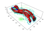
This is an example of how to create wind flow visualization in MATLAB®.
Read about the "isosurface", "isonormals", "isocaps", "coneplot", "streamline", "patch", and "reducepatch" functions in the MATLAB documentation.
For more examples, go to MATLAB Plot Gallery - http://www.mathworks.com/discovery/gallery.html
Cite As
MathWorks Plot Gallery Team (2026). MATLAB Plot Gallery - Wind (https://www.mathworks.com/matlabcentral/fileexchange/35250-matlab-plot-gallery-wind), MATLAB Central File Exchange. Retrieved .
General Information
- Version 1.1.0.2 (115 KB)
MATLAB Release Compatibility
- Compatible with any release
Platform Compatibility
- Windows
- macOS
- Linux
