Lab 1 - Digital Signal Processing. Sampling and Quantization
Exercise 2.1: Basic digital signals
(a) Write a MATLAB program to generate and display (using the stem function) the signals defined in
Table 1. The MATLAB code of the first signal (dirac) is given in the report template as an example.
(b) Write a MATLAB function [x, t] = sin_NU(f0, fs, T) to generate a sine signal. The output parameters x
and t are the signal and time vectors, respectively. The input parameters are f0 (signal frequency in
Hz), fs (sampling frequency in Hz), T (signal duration in sec.).
(c) Test your sin_NU function with the input parameter values .... and display the result using the plot function.
List of basic digital signals to generate:
- Dirac (Unit Response)
- Unit step (Heaviside step)
- Sign
- Rectangle
- Sine
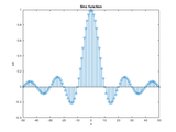
- Sine cardinal
Exercise 2.2: Audio aliasing
To illustrate the aliasing phenomenon, let’s perform two simple experiments allowing us to “hear” it. Using the sin_NU function of Exercise 1:
(a) Generate two 1 kHz sine signals (2 seconds duration), first signal at 20 kHz sample frequency and second signal at 1.5 kHz sample frequency;
(b) On the same graph, use the plot function to display the two signals versus t in the range 0 < t < 5 msec.;
(c) Listen to the two signals one after another using the function soundsc(x, fs); and
(d) Give your interpretation of this listening.
Exercise 2.3: Quantization
Quantization is done by replacing each value of an analog signal x(t) by the value of the nearest quantization level. To exemplify this operation, let’s simulate an unipolar ADC (Analog to Digital Converter) having the technical specifications: R = 10 Volts (full-scale range) and B = 3 (number of bits).
(a) Write a MATLAB function y = adc_NU(x, R, B) where x and y are vectors containing the input signal and the quantized signal, respectively;
(b) Test your function with an input ramp signal ranging from -5 to 15 Volts (1 volt per step); and
(c) On the same graph, use the plot and stem functions to display the input signal and quantized signal, respectively.
Cite As
Sanzhar Askaruly (2024). Lab 1 - Digital Signal Processing. Sampling and Quantization (https://www.mathworks.com/matlabcentral/fileexchange/54530-lab-1-digital-signal-processing-sampling-and-quantization), MATLAB Central File Exchange. Retrieved .
MATLAB Release Compatibility
Platform Compatibility
Windows macOS LinuxCategories
- Signal Processing > Signal Processing Toolbox >
- Reporting and Database Access > MATLAB Report Generator >
Tags
Community Treasure Hunt
Find the treasures in MATLAB Central and discover how the community can help you!
Start Hunting!Discover Live Editor
Create scripts with code, output, and formatted text in a single executable document.
Lab1_DigitalSignalProcessing/
| Version | Published | Release Notes | |
|---|---|---|---|
| 1.0.0.0 |
No major change made
|

