Modeling Market Risk Using Extreme Value Theory and Copulas
By Rick Baker, MathWorks
In the summer of 2002, flooding following a week of heavy rain in Europe caused billions of Euros in damage. Five years earlier, during the financial crisis in East Asia, a 75% drop in the Thai stock market contributed to a 554-point drop in the Dow Jones Industrial Average on October 27, 1997.
These apparently disparate events have at least three things in common: They occur rarely, they are extreme in scope, and they are difficult to predict. They are also typical of the kinds of events that statisticians must study in order to manage risk. For example, actuaries need to predict the likelihood and severity of a 100-year flood, while their colleagues in financial markets must assess the probability and magnitude of the next market crash.
Statisticians have applied a variety of techniques in their attempts to model rare events. These techniques frequently are based on Extreme Value Theory (EVT), a branch of statistics that analyzes events that deviate sharply from the norm, and copulas, which can be used to model the co-movement of dependent variables whose probability distributions are different from each other and might not be normal.
By combining EVT and t copulas, I illustrate an approach for modeling market risk and characterizing the behavior of portfolios during financial and economic crises. Using a global equity index portfolio as an example, this article shows how MATLAB, Statistics and Machine Learning Toolbox, and Optimization Toolbox enable you to apply this combined approach to evaluate a popular risk metric known as value-at-risk (VaR).
An Overview of the Process
Our approach enables us to model and simulate dependent stock returns consistent with historical performance. It comprises two distinct steps: a univariate modeling step and a multivariate modeling step.
Univariate Modeling
In the univariate step, we estimate a piecewise probability distribution for each variable using a nonparametric smoothing technique for the interior of the distribution. We apply EVT to better characterize the extreme values found at the upper and lower tails. When the first step is complete, we will have separate univariate models, one for each variable in our dataset. We will use these univariate distributions to transform the individual data of each index to the uniform probability scale, the form required to fit a copula.
Multivariate Modeling with a t Copula
In the multivariate step, we tie these separate models together using a t copula to take a multivariate, or portfolio-level, view to analyze the data.
A copula is a multivariate probability distribution whose individual variables are uniformly distributed. Copulas have experienced a tremendous surge in popularity in recent years. They enable analysts to isolate the dependence structure of portfolios from the description of the individual variables, and offer a compelling alternative to the traditional assumption of jointly normal portfolio returns.
By decoupling the univariate description of the individual variables from the multivariate description of the dependence structure, copulas offer significant theoretical and computational advantages over conventional risk management techniques.
Once these two steps are complete and the t copula has been calibrated, we can analyze any number of performance metrics on the risk model. For example, we can use Monte Carlo simulation to compute the VaR for an equally weighted portfolio over a one-month period.
Examining the Daily Closing Values of the Global Equity Index Data
In our example, the raw data consists of 1359 observations of daily adjusted closing values of the following representative equity indices spanning the trading dates February 5, 2001 to April 24, 2006: TSX Composite (Canada), CAC 40 (France), DAX (Germany), Nikkei 225 (Japan), FTSE 100 (U.K.), and S&P 500 (U.S.).
We use Datafeed Toolbox to download historical market data from Yahoo! Using Database Toolbox, we store the data for later analysis.
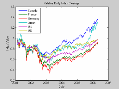
Figure 1 plots the relative value of each index. To better illustrate relative performance the initial value of each index has been normalized to unity .

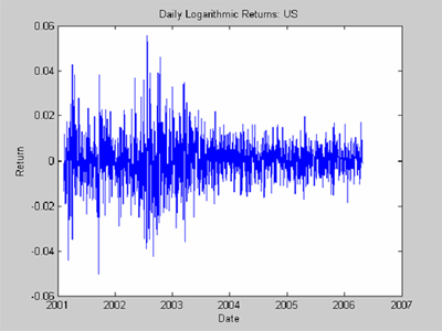
To prepare the data for subsequent modeling, we convert the daily closing values of each index to daily logarithmic returns (also called geometric, or continuously compounded, returns). The logarithmic returns for the U.S. index are shown in Figure 2. Logarithmic returns illustrate the extent of the day-to-day change in price: a positive spike represents a large daily gain, while a negative spike indicates a significant daily loss.

Filtering the Returns for Each Index with a GARCH Model
Before we can use EVT to model the tails of the distribution of an individual index, we must ensure that the data is approximately independent and identically distributed (iid).
A quick review of the index data reveals that it is not iid. For example, during the U.S. recessions in 2001 and 2002, there were wild swings in the stock market: Big gains one day were followed by big losses the next. During other periods, however, there was little volatility. This tendency reflects a degree of heteroskedasticity in which today’s volatility is dependent on yesterday’s volatility. Unless the data is preconditioned or filtered, this dependence will undermine the value of EVT.
To produce a series of iid observations, we use a GARCH model to filter out serial dependence in the data. Even though returns are not independent from one day to the next, the GARCH model produces a series of iid observations that let us more closely satisfy the requirements of EVT.
Estimating the Piecewise Probability Distributions
Once we have filtered the data, we fit a probability distribution to model the daily movements of each index. We do not assume that the data comes from a normal distribution or from any other simple parametric distribution. Rather, we want a more flexible empirical distribution that will let the data speak for itself.
A kernel density estimate works well for the interior of the distribution where most of the data is found, but it performs poorly when applied to the upper and lower tails. For risk management, it is essential to accurately characterize the tails of the distribution, even though the observed data in the tails is sparse. The generalized Pareto distribution (GPD) is often used for this purpose. In our example it will provide a reasonable model of the more extreme observations, large losses and large gains. Figure 3 shows the empirical cumulative distribution function (CDF) for the U.S. index, with the kernel density estimate for the interior and the GPD estimate for the upper and lower tails.
The underlying MATLAB code uses the Statistics and Machine Learning Toolbox function paretotails to automate the curve fit shown in Figure 3. We could perform a similar analysis interactively with the Distribution Fitting Tool GUI in Statistics and Machine Learning Toolbox.

Assessing the GPD Fit
Before repeating these steps for each index in the portfolio, we visually assess the results. Using the Statistics and Machine Learning Toolbox function gpfit, we use the data in the empirical CDF curve to find the parameters for the GPD in the tails of the curve. Figure 5 shows that the empirically generated CDF curve matches quite well with the fitted GPD results.

With the similarity of the curves providing a level of confidence in the results, we repeat the analysis for all six equity indices in the portfolio.
When the univariate step is complete, we will have six separate univariate models, one for each of the six indices, describing the distribution of daily gains and losses. But we still need to tie these separate models together, and that is what the copula model does.
Since a copula is a multivariate probability distribution whose individual variables are uniformly distributed, we can now use the univariate distributions that we just derived to transform the individual data of each index to the uniform scale, the form required to fit a copula.
Calibrating the t Copula
Extreme co-movement is a common phenomenon in the real world. For example, if the Canadian index is down 30 percent today, we can be fairly confident that the U.S. market suffered a relatively large decline as well. Modeling the indices with a Gaussian copula does not capture that behavior, because the most extreme events for the individual indices in a Gaussian copula model would be independent of each other. The t copula, on the other hand, includes a degrees-of-freedom parameter that can be used to model the tendency for extreme events to occur jointly.
We calibrate the t copula by estimating its scalar degrees-of-freedom parameter and its linear correlation matrix by maximum likelihood, using the Statistics and Machine Learning Toolbox function copulafit. This step accomplishes what estimating the piecewise CDF accomplished for a single index: it finds a model for the interaction between the indices, given models for the behavior of the individual indices.
Simulating Global Index Portfolio Returns with a t Copula
Once the calibration of the t copula is complete, the difficult part is over. We have calibrated the returns of each index independently based on EVT and then calibrated the dependence or co-movement between variables with the t copula. An analyst can use this complete model for a wide range of applications, such as calculating expected shortfall or performing dynamic portfolio analysis. We will use it to derive a measure of VaR.
Because we now have a probabilistic model that describes our observed data reasonably well, we can generate random daily returns that will be statistically equivalent to historical performance. Using Monte Carlo simulation, we can now analyze not just one historical trial but thousands. In MATLAB, we simulate 2000 independent random trials of dependent index returns over a holding period of one month, or 22 trading days. In this process, the GARCH Toolbox simulation engine is used to reintroduce the autocorrelation and heteroskedasticity observed in the original index returns.
After simulating the returns of each index and forming an equally weighted global portfolio, we use MATLAB to report the maximum gain and loss, as well as the VaR at various confidence levels, over the one-month risk horizon.
Figure 5 shows the empirical CDF of the simulated global portfolio returns over one month. VaR measures can be read directly from the curve. For instance, the 90 percent VaR, corresponding to 10 percent cumulative probability, is approximately -0.03. This means that, over the next month, we can be 90 percent confident that our portfolio will lose no more than 3 percent.

Advantages of this Approach
The two-step approach described in this article enables analysts to simulate and model dependent stock returns consistent with historical performance. The copula enables analysts to isolate the dependence structure of the portfolio from the description of the individual indices—a compelling alternative to the traditional assumption of jointly-normal portfolio returns.
By decoupling the univariate description of the individual variables from the multivariate description of the dependence structure, copulas offer significant theoretical and computational advantages over conventional risk management techniques.
Other Risk Modeling Applications
The value of modeling risk using EVT and t copulas extends to many different applications. In addition to measuring VaR and estimating potential flood damage, these techniques can be used by insurers to assess the likelihood of any number of natural disasters. They can also help organizations ensure compliance with the Basel Accords and other regulatory mandates that require financial institutions to quantify market risk and retain sufficient capital to protect against unanticipated losses.
Published 2007