lsimplot

Plot simulated time response of dynamic system to arbitrary inputs with additional plot customization options

Syntax

h = lsimplot(sys)

h = lsimplot(sys,u,t)

h = lsimplot(sys1,sys2,...,sysN,u,t)

h = lsimplot(sys1,LineSpec1,...,sysN,LineSpecN,u,t)

h = lsimplot(___,x0)

h = lsimplot(___,method)

h = lsimplot(AX,___)

h = lsimplot(___,plotoptions)

Description

lsimplot lets you plot simulated time response of dynamic system to arbitrary inputs with a broader range of plot customization options than lsim. You can use lsimplot to obtain the plot handle and use it to customize the plot, such as modify the axes labels, limits and units. You can also use lsimplot to draw a simulated time response plot on an existing set of axes represented by an axes handle. To customize an existing simulated time response plot using the plot handle:

1. Obtain the plot handle

2. Use getoptions to obtain the option set

3. Update the plot using setoptions to modify the required options

For more information, see Customizing Response Plots from the Command Line. To create simulated time response plots with default options or to extract simulated response data, use lsim.

h = lsimplot(sys) opens the Linear Simulation Tool for the dynamic system model sys, where you can interactively specify the driving input(s), the time vector, and initial state. It also returns the plot handle h. You can use this handle h to customize the plot with the getoptions and setoptions commands.

For more information about using the Linear Simulation Tool for linear analysis, see Working with the Linear Simulation Tool.

h = lsimplot(sys,u,t) plots the simulated time response of the model sys to the input signal u and the corresponding time vector t. For MIMO systems, u is a matrix with as many columns as the number of inputs and whose ith row specifies the input value at time t(i). For SISO systems, the input u can be specified either as a row or column vector.

h = lsimplot(sys1,sys2,...,sysN,u,t) plots the simulated response of multiple dynamic systems sys1,sys2,…,sysN using the input u and time vector t on the same plot. All systems must have the same number of inputs and outputs to use this syntax.

h = lsimplot(sys1,LineSpec1,...,sysN,LineSpecN,u,t) sets the line style, marker type, and color for the simulated time response of each system. All systems must have the same number of inputs and outputs to use this syntax.

h = lsimplot(___,x0) further specifies a vector x0 of initial state values, when sys is a state-space model.

h = lsimplot(___,method) specifies how lsimplot interpolates the input values between samples, when sys is a continuous-time model.

h = lsimplot(AX,___) plots the simulated response on the Axes object in the current figure with the handle AX.

h = lsimplot(___,plotoptions) plots the simulated response with the options set specified in plotoptions. You can use these options to customize the plot appearance using the command line. Settings you specify in plotoptions overrides the preference settings in the MATLAB^® session in which you run lsimplot. Therefore, this syntax is useful when you want to write a script to generate multiple plots that look the same regardless of the local preferences.

Examples

Customized Plot of Simulated Response to Arbitrary Input Signal

For this example, change time units to minutes and turn the grid on for the simulated response plot. Consider the following transfer function.

sys = tf(3,[1 2 3]);

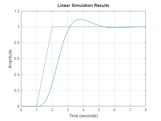
To compute the response of this system to an arbitrary input signal, provide lsimplot with a vector of the times t at which you want to compute the response and a vector u containing the corresponding signal values. For instance, plot the system response to a ramping step signal that starts at 0 at time t = 0, ramps from 0 at t = 1 to 1 at t = 2, and then holds steady at 1. Define t and compute the values of u.

t = 0:0.04:8;
u = max(0,min(t-1,1));

Use lsimplot plot the system response to the signal with a plot handle h.

h = lsimplot(sys,u,t);

The plot shows the applied input (u,t) in gray and the system response in blue.

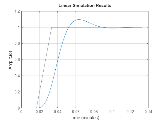
Use the plot handle to change the time units to minutes and to turn the grid on. To do so, edit properties of the plot handle, h using setoptions.

setoptions(h,'TimeUnits','minutes','Grid','on')

The plot automatically updates when you call setoptions.

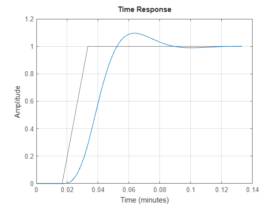
Alternatively, you can also use the timeoptions command to specify the required plot options. First, create an options set based on the toolbox preferences.

plotoptions = timeoptions('cstprefs');

Change properties of the options set by setting the time units to minutes and enabling the grid.

plotoptions.TimeUnits = 'minutes';
plotoptions.Grid = 'on';
lsimplot(sys,u,t,plotoptions);

Customized Plot Response of Multiple Systems to Same Input

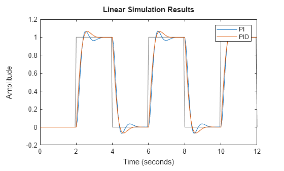
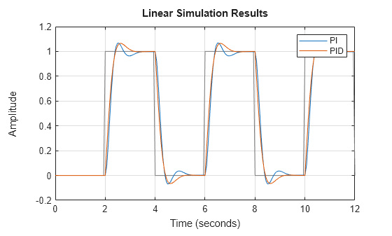
lsimplot allows you to plot the simulated responses of multiple dynamic systems on the same axis. For instance, compare the closed-loop response of a system with a PI controller and a PID controller. Then, customize the plot by enabling normalization and turning the grid on.

First, create a transfer function of the system and tune the controllers.

H = tf(4,[1 10 25]);
C1 = pidtune(H,'PI');
C2 = pidtune(H,'PID');

Form the closed-loop systems.

sys1 = feedback(H*C1,1);
sys2 = feedback(H*C2,1);

Plot the responses of both systems to a square wave with a period of 4 s.

[u,t] = gensig("square",4,12);
h1 = lsimplot(sys1,sys2,u,t);
legend("PI","PID")

Use setoptions to enable normalization and to turn on the grid.

setoptions(h1,'Normalize','on','Grid','on')

The plot automatically updates when you call setoptions.

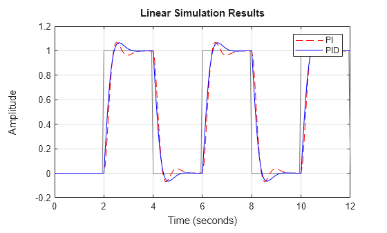
By default, lsimplot chooses distinct colors for each system that you plot. You can specify colors and line styles using the LineSpec input argument.

h2 = lsimplot(sys1,"r--",sys2,"b",u,t);
legend("PI","PID")
setoptions(h2,'Normalize','on','Grid','on')

The first LineSpec "r--" specifies a dashed red line for the response with the PI controller. The second LineSpec "b" specifies a solid blue line for the response with the PID controller. The legend reflects the specified colors and line styles.

Custom Plot of System Evolution from Initial Condition

By default, lsimplot simulates the model assuming all states are zero at the start of the simulation. When simulating the response of a state-space model, use the optional x0 input argument to specify nonzero initial state values. Consider the following two-state SISO state-space model.

A = [-1.5 -3;
      3   -1];
B = [1.3; 0];
C = [1.15 2.3];
D = 0;
sys = ss(A,B,C,D);

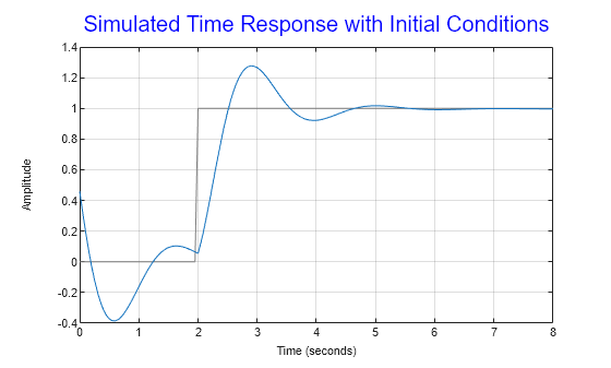
Suppose that you want to allow the system to evolve from a known set of initial states with no input for 2 s, and then apply a unit step change. Specify the vector x0 of initial state values, and create the input vector.

x0 = [-0.2 0.3];
t = 0:0.05:8;
u = zeros(length(t),1);
u(t>=2) = 1;

First, create a default options set using timeoptions.

plotoptions = timeoptions;

Next change the required properties of the options set plotoptions and plot the simulated response with the zero order hold option.

plotoptions.Title.FontSize = 15;
plotoptions.Title.Color = [0 0 1];
plotoptions.Grid = 'on';
h = lsimplot(sys,u,t,x0,plotoptions,'zoh');
hold on
title('Simulated Time Response with Initial Conditions')

The first half of the plot shows the free evolution of the system from the initial state values [-0.2 0.3]. At t = 2 there is a step change to the input, and the plot shows the system response to this new signal beginning from the state values at that time. Because plotoptions begins with a fixed set of options, the plot result is independent of the toolbox preferences of the MATLAB session.

Input Arguments

sys — Dynamic system

dynamic system model | model array

Dynamic system, specified as a SISO or MIMO dynamic system model or array of dynamic system models. Dynamic systems that you can use include:

• Continuous-time or discrete-time numeric LTI models, such as tf, zpk, or ss models.

• Sparse state-space models, such as sparss or mechss models. Final time tFinal must be specified when using sparse models.

• Generalized or uncertain LTI models such as genss or uss (Robust Control Toolbox) models. (Using uncertain models requires Robust Control Toolbox™ software.)

  • For tunable control design blocks, the function evaluates the model at its current value to plot the simulated response.

  • For uncertain control design blocks, the function plots the nominal value and random samples of the model.

• Identified LTI models, such as idtf (System Identification Toolbox), idss (System Identification Toolbox), or idproc (System Identification Toolbox) models. For identified models, you can also use the sim (System Identification Toolbox) command, which can compute the standard deviation of the simulated response and state trajectories. sim can also simulate all types of models with nonzero initial conditions, and can simulate nonlinear identified models.(Using identified models requires System Identification Toolbox™ software.)

lsimplot does not support frequency-response data models such as frd, genfrd, or idfrd models.

If sys is an array of models, the function plots the responses of all models in the array on the same axes.

LineSpec — Line style, marker, and color

character vector | string

Line style, marker, and color, specified as a character vector or string containing symbols. The symbols can appear in any order. You do not need to specify all three characteristics (line style, marker, and color). For example, if you omit the line style and specify the marker, then the plot shows only the marker and no line.

Example: '--or' is a red dashed line with circle markers

Line Style	Description
-	Solid line
--	Dashed line
:	Dotted line
-.	Dash-dot line

Marker	Description
'o'	Circle
'+'	Plus sign
'*'	Asterisk
'.'	Point
'x'	Cross
'_'	Horizontal line
'|'	Vertical line
's'	Square
'd'	Diamond
'^'	Upward-pointing triangle
'v'	Downward-pointing triangle
'>'	Right-pointing triangle
'<'	Left-pointing triangle
'p'	Pentagram
'h'	Hexagram

Color	Description
y	yellow
m	magenta
c	cyan
r	red
g	green
b	blue
w	white
k	black

u — Input signal for simulation

vector | array

Input signal for simulation, specified as a vector for single-input systems, and an array for multi-input systems.

• For single-input systems, u is a vector of the same length as t.

• For multi-input systems, u is an array with as many rows as there are time samples (length(t)) and as many columns as there are inputs to sys. In other words, each row u(i,:) represents the values applied at the inputs of sys at time t(i). Each column u(:,j) is the signal applied to the jth input of sys.

t — Time samples

vector

Time samples at which to compute the response, specified as a vector of the form 0:dT:Tf. The lsimplot command interprets t as having the units specified in the TimeUnit property of the model sys. The time vector must be real, finite, and must contain monotonically increasing and evenly spaced time samples.

For continuous-time systems, the lsimplot command uses the time step dT to discretize the model. If dT is too large relative to the system dynamics (undersampling), lsimplot issues a warning recommending a faster sampling time.

For discrete-time systems, the time step dT must equal the sample time of sys. Alternatively, you can omit t or set it to []. In that case, lsimplot sets t to a vector of the same length as u that begins at 0 with a time step equal to sys.Ts.

method — Discretization method

'zoh | 'foh'

Discretization method for sampling continuous-time models, specified as one of the following.

• 'zoh' — Zero-order hold

• 'foh' — First-order hold

When sys is a continuous-time model, lsimplot computes the time response by discretizing the model using a sample time equal to the time step dT = t(2)-t(1) of t. If you do not specify a discretization method, then lsimplot selects the method automatically based on the smoothness of the signal u. For more information about these two discretization methods, see Continuous-Discrete Conversion Methods.

x0 — Initial state values

vector of zeros (default) | vector

Initial state values for simulating a state-space model, specified as a vector having one entry for each state in sys. If you omit this argument, then lsim sets all states to zero at t = 0.

AX — Target axes

Axes object

Target axes, specified as an Axes object. If you do not specify the axes and if the current axes are Cartesian axes, then stepplot plots on the current axes. Use AX to plot into specific axes when creating a step plot.

plotoptions — Step plot options set

TimePlotOptions object

Step plot options set, specified as a TimePlotOptions object. You can use this option set to customize the step plot appearance. Use timeoptions to create the option set. Settings you specify in plotoptions overrides the preference settings in the MATLAB session in which you run stepplot. Therefore, plotoptions is useful when you want to write a script to generate multiple plots that look the same regardless of the local preferences.

For the list of available options, see timeoptions.

Output Arguments

h — Plot handle

handle object

Plot handle, returned as a handle object. Use the handle h to get and set the properties of the simulated response plot using getoptions and setoptions. For the list of available options, see the Properties and Values Reference section in Customizing Response Plots from the Command Line.

Version History

Introduced before R2006a