R2023a

New Features, Bug Fixes, Compatibility Considerations

Apps and Visualization

Experiment Manager: Create visualizations for custom training experiments

You can now display visualizations for your custom training experiments directly in the Experiment Manager app. When the training is complete, the Review Results gallery in the toolstrip displays a button for each figure that you create in your training function. To display a figure in the Visualizations pane, click the corresponding button in the Custom Plot section of the gallery. For examples of custom training experiments with visualizations, see:

• Use Bayesian Optimization in Custom Training Experiments

• Run a Custom Training Experiment for Image Comparison

• Use Experiment Manager to Train Generative Adversarial Networks (GANs)

• Custom Training with Multiple GPUs in Experiment Manager

Experiment Manager: Debug code before or after running experiment

Diagnose problems in your experiment directly from the Experiment Manager app.

• Before you run an experiment, you can debug your setup and training functions using your choice of hyperparameter values.

• After you run an experiment, you can debug your setup and training functions using the same random seed and hyperparameter values you use in one of your trials.

You can add breakpoints, inspect the values of your variables, and step through the code line by line. For more information, see Debug Code Before and After Running Experiments.

Experiment Manager: Specify constraints and acquisition function for Bayesian optimization

You can now specify deterministic constraints, conditional constraints, and an acquisition function for experiments that use Bayesian optimization. Under Bayesian Optimization Options, click Advanced Options and specify these fields:

• Deterministic Constraints

• Conditional Constraints

• Acquisition Function Name

For more information about these options, see Deterministic Constraints — XConstraintFcn (Statistics and Machine Learning Toolbox), Conditional Constraints — ConditionalVariableFcn (Statistics and Machine Learning Toolbox), and Acquisition Function Types (Statistics and Machine Learning Toolbox).

Experiment Manager: Load preconfigured templates for audio classification

If you have an Audio Toolbox™ license, you can now set up your built-in or custom training experiments for audio classification by selecting a preconfigured template in Experiment Manager.

Deep Network Designer: View and edit custom layer class files

You can now view and edit custom layer class files from Deep Network Designer. To view a custom layer class definition, select the layer and then click Edit Class Layer in the Properties pane. The layer class file opens in the MATLAB^® Editor. For an example that shows how to view a custom layer class definition in Deep Network Designer, see View Autogenerated Custom Layers Using Deep Network Designer.

Deep Network Designer: Create and edit function layers

You can now create and edit function layers in Deep Network Designer. For more information about function layers, see functionLayer.

Deep Network Designer: User interface improvements

Deep Network Designer has improved user interfaces for importing data and specifying training options. Use expandable training option groups to easily find and edit the training options that you need.

 Functionality being removed or changed

plotv will be removed

Still runs

plotv will be removed in a future release. Use plot instead. These functions have several differences that require updates to your code. For example, let M be a matrix containing three two-element vectors.

M = [-0.4 0.7 0.2 ;
     -0.5 0.1 0.5];

Plot the column vectors as lines from the origin.

Using plotv	Using plot
plotv(M,'-')	origin = zeros(1,size(M,2)); plot([origin; M(1,:)],[origin; M(2,:)]);

Algorithms

Self-Attention Layer: Create networks with self-attention layers

Create networks that contain self-attention layers using selfAttentionLayer. A self-attention layer computes the single-head and multihead self-attention of the input.

The layer performs these steps:

1. Compute the queries, keys, and values from the input.

2. Compute the scaled dot-product attention across different heads using the queries, keys, and values.

3. Merge the results from the heads.

4. Perform a linear transformation on the merged result.

Layer Normalization: Specify dimensions to normalize over

When you use layerNormalizationLayer objects or the layernorm function, specify the dimension to normalize over using the OperationDimension option.

Normalization: Specify lower values for variance offset

The Epsilon property of BatchNormalizationLayer, GroupNormalizationLayer, InstanceNormalizationLayer, and LayerNormalizationLayer objects now supports positive values less than 1e-5.

The Epsilon name-value argument of the batchnorm, groupnorm, instancenorm, and layernorm functions now supports positive values less than 1e-5.

In previous releases, the value of Epsilon must be greater than or equal to 1e-5.

Gated Recurrent Units: Specify reset gate mode for dlnetwork and dlarray objects

For gruLayer objects in dlnetwork objects, or when you apply the gru operation to dlarray objects, set ResetGateMode to one of these values:

• "after-multiplication" — Apply the reset gate after matrix multiplication. This option is cuDNN compatible.

• "before-multiplication" — Apply the reset gate before matrix multiplication.

• "recurrent-bias-after-multiplication" — Apply the reset gate after matrix multiplication and use an additional set of bias terms for the recurrent weights.

For more information about the reset gate calculations, see Gated Recurrent Unit Layer.

Neural ODEs: Characterize ODE system using neural network

When you use the dlode45 function, characterize a system of ODEs as a neural network by specifying a dlnetwork object as the first input argument net.

In previous releases, you must specify ODE systems as a function handle. Starting in R2023a, if you specify the ODE function as a function handle, then you can also specify learnable parameters theta as one of these values:

• A dlnetwork object

• A cell array of dlnetwork and dlarray objects

• A structure of dlnetwork and dlarray objects or nested structures of dlnetwork and dlarray objects

L-BFGS Solver: Train neural network using L-BFGS solver

Train networks using a custom training loop with the limited-memory BFGS (L-BFGS) algorithm using the lbfgsupdate function and lbfgsState objects.

The L-BFGS algorithm is a quasi-Newton method that approximates the Broyden-Fletcher-Goldfarb-Shanno (BFGS) algorithm. The L-BFGS algorithm is best suited for small networks and data sets where you can process the data set in a single batch.

For an example that shows how to train a physics-informed neural network (PINN) to numerically compute the solution of the Burgers equation using the L-BFGS algorithm, see Solve Partial Differential Equation with L-BFGS Method and Deep Learning.

Automatic Differentiation: Calculate standard deviation of dlarray objects

Calculate the standard deviation of dlarray objects using the std function. For a full list of functions that support dlarray input, see List of Functions with dlarray Support.

MEX Acceleration: Accelerate prediction using networks with numeric feature input

The name-value option Acceleration="mex" of the activations, classify, and predict functions now supports networks containing FeatureInputLayer objects.

MEX acceleration is available only when you use a GPU. Using a GPU requires a Parallel Computing Toolbox™ license and a supported GPU device. For information about supported devices, see GPU Computing Requirements (Parallel Computing Toolbox).

Parameter Updates: Improved performance of parameter updates using a GPU

Parameter updates on the GPU show improved performance, including parameter updates using the adamupdate, sgdmupdate, and rmspropupdate functions. For example, updating parameters using adamupdate in this test is about 1.4x faster than in the previous release:

function timeAdamUpdate

% Prepare network.
net = resnet101;
lgraph = layerGraph(net);
lgraph = removeLayers(lgraph,lgraph.Layers(end).Name);
net = dlnetwork(lgraph);

% Convert the learnable parameters to gpuArray objects.
net = dlupdate(@gpuArray,net);

% Initialize the update variables.
fakeG = net.Learnables;
avgG = [];
avgsqG = [];
[net,avgG,avgsqG] = adamupdate(net,fakeG,avgG,avgsqG,1);

% Warm-up iterations.
for idx=1:10
    adamupdate(net,fakeG,avgG,avgsqG,2);
end

% Time adamupdate.
gputimeit(@() adamupdate(net,fakeG,avgG,avgsqG,2))

end

The approximate execution times are:

R2022b: 0.34 seconds

R2023a: 0.25 seconds

The code was timed on a Windows^® 10, Intel^® Xeon^® W-2133 @ 3.60 GHz test system with an NVIDIA^® RTX A5000 GPU by calling the timeAdamUpdate function.

Accessing dlnetwork Learnables: Improved performance

Accessing the learnable parameters of a dlnetwork object shows improved performance. For example, accessing the learnable parameters of a trained network is about 2.1x faster than in the previous release.

function timeGetLearnables

% Prepare network.
net = resnet101;
lgraph = layerGraph(net);
lgraph = removeLayers(lgraph,lgraph.Layers(end).Name);
net = dlnetwork(lgraph);

% Time getting learnables from network.
tic
for n = 1:100
    net.Learnables;
end
toc

end

The approximate execution times are:

R2022b: 0.53 seconds

R2023a: 0.25 seconds

The code was timed on a Windows 10, Intel Xeon W-2133 @ 3.60 GHz test system with an NVIDIA RTX A5000 GPU by calling the timeGetLearnables function.

crossentropy Function: Improved performance within dlgradient call

The crossentropy function shows improved performance when used within a dlgradient call. For example, evaluating gradients of the cross-entropy loss on the GPU in the following test is about 1.8x faster than in the previous release:

function timeCrossEntropy

% Prepare input data and gradient function.
x = dlarray(randn(5000,"gpuArray"),"SS");
y = dlarray(randn(5000,"gpuArray"));
CE = @(x,y) dlgradient(crossentropy(x,y),{x,y});

% Warm-up iterations.
for i = 1:10
    dlfeval(CE,x,y);
end

% Timed iterations.
tic
for i = 1:10
    dlfeval(CE,x,y);
end
toc

end

The approximate execution times are:

R2022b: 0.21 seconds

R2023a: 0.12 seconds

The code was timed on a Windows 10, Intel Xeon W-2133 @ 3.60 GHz test system with an NVIDIA RTX A5000 GPU by calling the timeCrossEntropy function.

Accelerated Functions: Improved performance

Functions accelerated using dlaccelerate show improved performance. For example, making the first prediction with a network where the predict function has been accelerated using dlaccelerate in the following test is about 2.3x faster than in the previous release:

function timeFirstAcceleratedFunction

% Prepare network.
vectorInputSize =  [28 1 1];
outSize = 4;
layers = [
    imageInputLayer(vectorInputSize,Normalization="none")
    fullyConnectedLayer(256)
    reluLayer
    fullyConnectedLayer(128)
    reluLayer
    fullyConnectedLayer(64)
    reluLayer
    fullyConnectedLayer(32)
    reluLayer
    fullyConnectedLayer(outSize)];
net = dlnetwork(layers);

% Prepare input data.
X = dlarray(rand([28 1 1],"gpuArray"),"SSC");

% Prepare accelerated function.
accFcn = dlaccelerate(@(net,X) predict(net,X));

% Time accelerated function.
tic
for i=1:100
    clearCache(accFcn);
    accFcn(net,X);
end
toc

end

The approximate execution times are:

R2022b: 6.65 seconds

R2023a: 2.86 seconds

The code was timed on a Windows 10, Intel Xeon W-2133 @ 3.60 GHz test system with an NVIDIA RTX A5000 GPU by calling the timeFirstAcceleratedFunction function.

Making subsequent predictions with a network where the predict function has been accelerated using dlaccelerate in this test is about 1.5x faster than in the previous release:

function timeAcceleratedFunction

% Prepare network.
vectorInputSize =  [28 1 1];
outSize = 4;
layers = [
    imageInputLayer(vectorInputSize,Normalization="none")
    fullyConnectedLayer(256)
    reluLayer
    fullyConnectedLayer(128)
    reluLayer
    fullyConnectedLayer(64)
    reluLayer
    fullyConnectedLayer(32)
    reluLayer
    fullyConnectedLayer(outSize)];
net = dlnetwork(layers);

% Prepare input data.
X = dlarray(rand([28 1 1],"gpuArray"),"SSC");

% Prepare accelerated function.
accFcn = dlaccelerate(@(net,X) predict(net,X));

% Warm-up iterations.
for n = 1:10
    accFcn(net,X);
end

% Timed iterations.
tic
for n = 1:100
    accFcn(net,X);
end
toc

end

The approximate execution times are:

R2022b: 0.15 seconds

R2023a: 0.11 seconds

The code was timed on a Windows 10, Intel Xeon W-2133 @ 3.60 GHz test system with an NVIDIA RTX A5000 GPU by calling the timeAcceleratedFunction function.

dlnetwork Training with Validation: Improved performance when training and validating a network

Training a dlnetwork object while performing validation shows improved performance. For example, training a network and validating the network using the predict in the following test is about 14.9x faster than in the previous release:

function timeTrainingWithValidation

% Prepare network.
net = resnet50;
lgraph = layerGraph(net);
lgraph = removeLayers(lgraph,lgraph.Layers(end).Name);
net = dlnetwork(lgraph);

% Prepare input data.
X = dlarray(gpuArray.randn([net.Layers(1).InputSize 32],"single"),"SSCB");

% Prepare training functions.
lossFcn = @(z)sum(z,'all');
gradFcn = @(n,x)dlgradient(lossFcn(forward(n,x)),n.Learnables);
trainFcn = @(n,x)dlfeval(gradFcn, n, x);

% Warm-up iterations.
gpu = gpuDevice;
wait(gpu);
for i=1:3
    net = adamupdate(net, trainFcn(net,X),[],[],i);
    predict(net,X);
end

% Timed iterations.
wait(gpu)
tic
for i = 1:10
    net = adamupdate(net,trainFcn(net,X),[],[],i);
    predict(net,X);
end
wait(gpu)
toc

end

The approximate execution times are:

R2022b: 71.4 seconds

R2023a: 4.8 seconds

The code was timed on a Windows 10, Intel Xeon W-2133 @ 3.60 GHz test system with an NVIDIA RTX A5000 GPU by calling the timeTrainingWithValidation function.

dlnetwork Inference: Improved performance of GPU inference on networks performing operations with a stride

GPU inference using a dlnetwork object containing layers performing operations with a stride shows improved performance. Layers that perform operations with a stride include convolution and pooling layers, such as a convolution2dLayer and a maxPooling2dLayer, when any element of the stride property is greater than 1. The performance improvement is greater for networks containing more layers that perform operations with a stride. For example, making predictions using resnet101 on the GPU in the following test is about 1.5x faster than in the previous release:

function timeStrideInference

% Load a trained network.
net = resnet101;
lgraph = layerGraph(net);
lgraph = removeLayers(lgraph,lgraph.Layers(end).Name);
net = dlnetwork(lgraph);

% Prepare input data.
X = rand(224,224,3,150,"gpuArray");
dlX = dlarray(X,"SSCB");

% Time the predict function.
gputimeit(@() predict(net,dlX))

end

The approximate execution times are:

R2022b: 0.16 seconds

R2023a: 0.11 seconds

The code was timed on a Windows 10, Intel Xeon W-2133 @ 3.60 GHz test system with an NVIDIA RTX A5000 GPU by calling the timeStrideInference function.

dlnetwork Inference: Improved performance of inference on branching networks

Computing the output of a layer in a branch of a dlnetwork object where other branches are not needed shows improved performance. For example, computing the output of a layer in one branch of a network in the following test is about 1.4x faster than in the previous release:

function timeBranchInference

% Prepare network.
net = nasnetlarge; 
lgraph = layerGraph(net);
lgraph = removeLayers(lgraph,lgraph.Layers(end).Name);
net = dlnetwork(lgraph);
inputSize = net.Layers(1).InputSize; 

% Prepare input data.
X = rand([inputSize 1]);
X = dlarray(X,"SSCB"); 

% Time computing the output of layer normal_add_4_0.
timeit(@() predict(net,X,Outputs="normal_add_4_0"))

end

The approximate execution times are:

R2022b: 0.19 seconds

R2023a: 0.14 seconds

The code was timed on a Windows 10, Intel Xeon W-2133 @ 3.60 GHz test system with an NVIDIA RTX A5000 GPU by calling the timeBranchInference function.

dlnetwork Inference: Improved performance for networks containing the layer sequence convolution, addition, ReLU

Inference using a dlnetwork object containing the layer sequence convolution, addition, ReLU shows improved performance. For example, inference on the network in the following test is about 1.3x faster than in the previous release:

function timeConvAddReLU

% Prepare network containing Conv-Add-ReLU sequence.
layers = [
    imageInputLayer([28 28 1],Normalization="none")
    convolution2dLayer(5,20)
    reluLayer(Name="relu_1")
    convolution2dLayer(3,20,Padding=1)
    reluLayer
    convolution2dLayer(3,20,Padding=1)
    additionLayer(2,Name="add")
    reluLayer
    fullyConnectedLayer(10)
    softmaxLayer];
 
lgraph = layerGraph(layers);
lgraph = connectLayers(lgraph,"relu_1","add/in2");
 
net = dlnetwork(lgraph);
 
% Prepare input data.
[XTest,TTest] = digitTest4DArrayData;
XTest = dlarray(gpuArray(XTest),"SSCB"); 

% Warm-up iterations.
for idx=1:40
YPred = predict(net,XTest);
end
 
% Time predict function. 
gputimeit(@() predict(net,XTest))

end

The approximate execution times are:

R2022b: 9.5 milliseconds

R2023a: 7.6 milliseconds

The code was timed on a Windows 10, AMD^® EPYC 8-Core Processor @ 3.20 GHz test system with an NVIDIA RTX A5000 GPU by calling the timeConvAddReLU function.

Custom Layers: Improved performance in a dlnetwork

Custom layers with a custom backward method show improved performance for dlnetwork training and inference. For example, computing the network outputs for training using forward for a network containing a number of instances of a custom ReLU layer in this test is about 4.6x faster than in the previous release:

function timeCustomWithBackward

% Create network containing 100 custom layers.
layer = reluLayerWithBackward;
layerArray = repelem(layer,100);
dlnet = dlnetwork(layerArray,dlarray(1,"SSCB"));

% Prepare input data.
x = dlarray(1,"SSCB");

% Warm-up iterations.
for i=1:1000
    forward(dlnet,x);
end

% Timed iterations.
tic;
for i=1:1000
    forward(dlnet,x);
end
toc

end

The approximate execution times are:

R2022b: 60.27 seconds

R2023a: 13.06 seconds

The code was timed on a Windows 10, Intel Xeon W-2133 @ 3.60 GHz test system with an NVIDIA RTX A5000 GPU by calling the timeCustomWithBackward function with the following custom layer reluLayerWithBackward on the path.

classdef reluLayerWithBackward < nnet.layer.Layer
    % reluLayerWithBackward - A custom layer that implements ReLU.
    % The input to reluLayer is expected to have one channel.

    properties
        ValidInputSize = [4 5 3 10]
        ValidObsDim = 2
    end

    methods
        function layer = reluLayerWithBackward(varargin)
            ip = inputParser;
            ip.addParameter(Name="relu");
            ip.parse(varargin{:});
            layer.Name = ip.Results.Name;
        end

        function Z = predict(~,X)
            % Forward input data through the layer and output the result.
            Z = max(0,X);
        end

        function dLdX = backward(~,X,~,dLdZ,~)
            % Backpropagate the derivative of the loss function through
            % the layer.
            dLdX = dLdZ .* (X >= 0);
        end
    end
end

 Functionality being removed or changed

layerNormalizationLayer normalizes over channel and spatial dimensions of sequence data

Behavior change

Starting in R2023a, by default, layerNormalizationLayer normalizes sequence data over the channel and spatial dimensions. In previous versions, the software normalizes over all dimensions except for the batch dimension (the spatial, time, and channel dimensions). Normalization over the channel and spatial dimensions is usually better suited for this type of data. To reproduce the previous behavior, set OperationDimension to "batch-excluded".

layernorm normalizes over channel and spatial dimensions of 2-D and 3-D image sequence data

Behavior change

Starting in R2023a, by default, layernorm normalizes 2-D and 3-D image sequence data over the channel and spatial dimensions. In previous versions, the software normalizes over all dimensions except for the batch dimension (the spatial, time, and channel dimensions). Normalization over the channel and spatial dimensions is usually better suited for these types of data. To reproduce the previous behavior, set OperationDimension to "batch-excluded".

layernorm normalizes over channel dimension of 1-D image, vector sequence, and 1-D image sequence data

Behavior change

Starting in R2023a, by default, layernorm normalizes 1-D image data (data with one spatial dimension and no time dimension), vector sequence (data with a time dimension and no spatial dimensions) and 1-D image sequence data (data with one spatial dimension and a time dimension) over the channel dimension. In previous versions, the software normalizes over all dimensions except for the batch dimension (the spatial, time, and channel dimensions). Normalization over the channel dimension is usually better suited for these types of data. To reproduce the previous behavior, set OperationDimension to "batch-excluded".

Custom layer resetState function must set learnable and state properties only

Behavior change

The custom layer resetState function must not set any layer properties except for learnable and state properties. If the function sets other layer properties, then the layer can behave unexpectedly. For more information, see Define Custom Deep Learning Intermediate Layers.

functionToLayerGraph will be removed

Warns

functionToLayerGraph will be removed in a future release. Construct layer graphs manually instead. For a list of layers, see List of Deep Learning Layers. For information about developing custom layers, see Define Custom Deep Learning Layers.

Deployment

Quantization: Quantize dlnetwork objects

The dlquantizer object and Deep Network Quantizer now support dlnetwork objects for quantization with the quantize function.

After you create a quantized dlnetwork object, perform inference on the network using the predict function.

Quantization: Quantize yolov3ObjectDetector and yolov4ObjectDetector using dlquantizer

You can now quantize the yolov3ObjectDetector (Computer Vision Toolbox) and yolov4ObjectDetector (Computer Vision Toolbox) objects using dlquantizer.

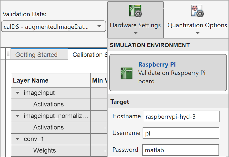
Quantization: Specify Raspberry Pi as target for quantization

You can now specify a raspi object as the target for quantization using the Target property of dlquantizationOptions when you set the dlquantizer ExecutionEnvironment property to "CPU".

In the Deep Network Quantizer app, you can now specify an existing raspi object as the target or create a new Raspberry Pi^® connection using the Hardware Settings option. For an example of quantized network validation on an CPU using the Deep Network Quantizer app, see Quantize a Network for CPU Deployment.

Quantized TensorFlow Lite Models: Configure predict function to accept and return fp32 values

Quantized deep learning models use reduced-precision numbers, usually 8-bit integers (with the int8 or uint8 data type) instead of 32-bit floating point numbers (with the fp32 data type), to represent the model parameters. For inference computation with quantized TFLite models, the predict function accepts and returns 8-bit integer values by default. In R2023a, when you perform inference computation with quantized TFLite models, you can configure the predict function to accept and return fp32 values and perform the appropriate conversion at the function interface. To do this, use the predict function with the additional name-value arguments QuantizeInputs and DequantizeOutputs.

TensorFlow Lite: Use newer version of TensorFlow Lite library in simulation and code generation

In R2023a, you can perform inference with models created using TFLite version 2.8.0 in simulation and code generation. TFLite models are forward and backward compatible. So, if your model was created using a different version of the library but contains layers that are available in version 2.8.0, you can still simulate, generate code for, and deploy your model. For more information, see Prerequisites for Deep Learning with TensorFlow Lite Models.

 Functionality being removed or changed

Specify Raspberry Pi as target for quantization using the Target property of dlquantizationOptions

Behavior change

Starting from R2023a, you must specify a raspi object as the target for quantization using the Target property of dlquantizationOptions. In previous releases, you must set the quantization target as Raspberry Pi and the software uses the most recent raspi connection when you set the ExecutionEnvironment property of the dlquantizer object to "CPU".

Interoperability

PyTorch Layer Support: Import networks that include multiple new layers

You can now import a PyTorch^® network that includes these layers:

• torch.nn.Conv1d

• torch.nn.ConvTranspose1d

• torch.nn.GroupNorm

• torch.nn.LayerNorm

• torch.nn.PReLU

• torch.nn.SiLU

• torch.nn.Softmax

• torch.nn.Upsample (2-D image)

• torch.nn.UpsamplingNearest2d

• torch.nn.UpsamplingBilinear2d

For a full list of supported layers, see Conversion of PyTorch Layers and Functions into Built-In MATLAB Layers and Functions.

PyTorch Function Support: Import networks that include multiple new functions

You can now import a PyTorch network that includes these functions:

• torch.nn.functional.avg_pool2d

• torch.nn.functional.conv1d

• torch.nn.functional.conv2d

• torch.nn.functional.log_softmax

• torch.nn.functional.max_pool2d

• torch.nn.functional.relu

• torch.nn.functional.silu

• torch.nn.functional.softmax

For a full list of supported functions, see Conversion of PyTorch Layers and Functions into Built-In MATLAB Layers and Functions.

PyTorch Operator Support: Import networks that include multiple new operators

You can now import a PyTorch network that includes these operators:

• Mathematical Operators

  • torch.argmax

  • torch.bmm

  • torch.matmul

  • torch.max

  • torch.permute

  • torch.pow

  • torch.split

  • torch.stack

  • torch.sum

  • torch.squeeze

  • torch.unsqueeze

  • torch.zeros

• Matrix Operators

  • torch.tensor.expand

  • torch.tensor.expand_as

For a full list of supported operators, see Conversion of PyTorch Layers and Functions into Built-In MATLAB Layers and Functions.

PyTorch Model Support: Extended model support for PyTorch importer

You can now import image segmentation models using the importNetworkFromPyTorch function.

PyTorch Version Support: Updated support for PyTorch

The importNetworkFromPyTorch function now fully supports PyTorch version 1.10.0.

TensorFlow Export Layer Support: Export networks that include multiple new layers

You can now export a trained MATLAB deep learning network that includes point cloud input, depth to space, space to depth, 2-D resize, and 3-D resize layers to the TensorFlow™ model format by using exportNetworkToTensorFlow. For a full list of supported layers, see Layers Supported for Exporting to TensorFlow .

TensorFlow Export Model Support: Enhanced Support for layer normalization layer

exportNetworkToTensorFlow now requires the TensorFlow module tfa for a MATLAB network or layer graph that contains a layerNormalizationLayer object only when you set the OperationDimension property of the layer to "batch-excluded".

TensorFlow Import Operator Support: Import networks that include multiple new operators

You can now import a TensorFlow network that includes these operators using the importTensorFlowNetwork and importTensorFlowLayers functions:

• All

• Equal

• Fill

• Greater

• NonMaxSuppressionV5

• ResizeBilinear

• Select

• Slice

• Split

• Sum

• Unpack

• Where

For a list of TensorFlow operators that the functions support for conversion into MATLAB functions with dlarray support, see Supported TensorFlow Operators.

ONNX Export Layer Support: Export networks that include 3-D global average pooling and 3-D global max pooling layers

You can now export a trained MATLAB deep learning network that includes globalAveragePooling3dLayer and globalMaxPooling3dLayer objects to the ONNX™ model format by using exportONNXNetwork. For a full list of supported layers, see Layers Supported for ONNX Export.

ONNX Export Layer Support: Export networks that include point cloud input layer

You can now export a trained MATLAB deep learning network that includes a point cloud input layer to the ONNX model format by using exportONNXNetwork. For a full list of supported layers, see Layers Supported for ONNX Export.

 Functionality being removed or changed

importTensorFlowNetwork and importTensorFlowLayers create a custom layer for TensorFlow-Keras Concatenate layer

Behavior change

The importTensorFlowNetwork and importTensorFlowLayers functions return an autogenerated custom layer for the TensorFlow-Keras Concatenate layer instead of the built-in Deep Learning Toolbox™ concatenationLayer or depthConcatenationLayer objects. In previous releases, the functions use concatenationLayer or depthConcatenationLayer objects and assume a concatenation dimension based on the input layer of the network being imported. However, for some complex networks, this assumption is not true. Therefore, the software uses an autogenerated custom layer to perform the concatenation. The autogenerated custom layer ensures the correct translation of the TensorFlow-Keras Concatenate layer into MATLAB at run time.

Verification

Out-of-Distribution Detection: Identify out-of-distribution inputs

Out-of-distribution (OOD) detection is the process of identifying inputs to a deep neural network that can cause the network to behave unexpectedly. This type of input can occur when a model is given data that is different from the data used to train it. For example, data collected in a different way, at a different time, under different conditions, or for a different task than the data on which the model was originally trained. By assigning confidence scores to the predictions of a network, you can classify data as in-distribution (ID) or OOD.

Use the networkDistributionDiscriminator function to create a distribution discriminator. The function finds a threshold to separate ID and OOD data using requirements on the true positive or false positive goal. You can also compute the distribution confidence scores using the baseline, ODIN energy, or HBOS method. You can use the distributionScores function with the returned object to find the distribution confidence scores for a specified input.

To use the discriminator to classify data as ID or OOD, use the discriminator as the first input to the isInNetworkDistribution function. The isInNetworkDistribution function also supports providing a trained classification network as the first input argument. This syntax is simpler but does not have the flexibility of using a discriminator object, which you can use to specify additional options and to automatically tune the threshold.

For examples that show how to detect OOD data, see Out-of-Distribution Detection for Deep Neural Networks and Out-of-Distribution Data Discriminator for YOLO v4 Object Detector.

These functions require the AI Verification Library for Deep Learning Toolbox support package. To download and install the support package, use the Add-On Explorer. Alternatively, see AI Verification Library for Deep Learning Toolbox.

Formal Methods: Test robustness and estimate output bounds of convolutional neural networks

The verifyNetworkRobustness and estimateNetworkOutputBounds functions now support networks with these layers:

• batchNormalizationLayer

• convolution2dLayer

• averagePooling2dLayer

• globalAveragePooling2dLayer

• dropoutLayer

• sigmoidLayer

The verifyNetworkRobustness and estimateNetworkOutputBounds functions require the AI Verification Library for Deep Learning Toolbox support package. To download and install the support package, use the Add-On Explorer. Alternatively, see AI Verification Library for Deep Learning Toolbox.

Out-of-Distribution Detection: Detect out-of-distribution data using mini-batches (June 2023; Version 23.1.1)

The networkDistributionDiscriminator, isInNetworkDistribution, and distributionScores functions now support minibatchqueue objects. You can use minibatchequeue objects to create, preprocess, and manage mini-batches of data, and to automatically convert your data to a dlarray object.

Out-of-Distribution Detection: Display out-of-distribution detection progress information (June 2023; Version 23.1.1)

You can now view progress information when detecting out-of-distribution data and creating a data discriminator. To view the progress information, set the VerbosityLevel option when you use the networkDistributionDiscriminator, isInNetworkDistribution, and distributionScores functions. The software displays progress information in the Command Window. You can set the VerbosityLevel to "off", "summary", or "detailed".

Formal Methods: Verify more types of layers (June 2023; Version 23.1.1)

The verifyNetworkRobustness and estimateNetworkOutputBounds functions now support networks containing these layers:

• maxPooling2dLayer — 2-D max pooling layer

• globalMaxPooling2dLayer — 2-D global max pooling layer

• nnet.onnx.layer.ElementwiseAffineLayer — ONNX built-in layer

The verifyNetworkRobustness and estimateNetworkOutputBounds functions also support imageInputLayer and featureInputLayer layers with the Normalization option set to "zerocenter", "zscore", "rescale-symmetric", "rescale-zero-one", or "none". Custom normalization functions are not supported. Previously, the functions only supported these layers with the Normalization option set to "none".

Out-of-Distribution Detection: Code generation support for out-of-distribution detection (June 2023; Version 23.1.1)

These out-of-distribution detection functions and objects now support C, C++, and CUDA^® code generation:

• networkDistributionDiscriminator

• distributionScores

• isInNetworkDistribution

• BaselineDistributionDiscriminator

• EnergyDistributionDiscriminator

• HBOSDistributionDiscriminator

• ODINDistributionDiscriminator

To load a network distribution discriminator for code generation, use the coder.loadNetworkDistributionDiscriminator function.

These functions require the AI Verification Library for Deep Learning Toolbox support package. To download and install the support package, use the Add-On Explorer. Alternatively, see AI Verification Library for Deep Learning Toolbox.

Application Examples

Deep Learning Workflows: New and updated examples and topics

Use these new examples and topics to progress with deep learning:

• Work with Deep Learning Data in Azure Blob Storage

• Train Sequence Classification Network Using Custom Training Loop

• Out-of-Distribution Detection for Deep Neural Networks

• Quantization Aware Training (GitHub)

• Out-of-Distribution Data Discriminator for YOLO v4 Object Detector

• Explore Quantized Semantic Segmentation Network Using Grad-CAM

• Quantize Semantic Segmentation Network and Generate CUDA Code

• Detect Issues During Deep Neural Network Training

• Reduced Order Modeling Using Continuous-Time Echo State Network

• Solve Partial Differential Equation with L-BFGS Method and Deep Learning

Image Processing and Computer Vision: New examples

Use these new examples for image processing and computer vision tasks:

• Detect Defects on Printed Circuit Boards Using YOLO v4 Network

• Cardiac Left Ventricle Segmentation from Cine-MRI Images Using U-Net Network

Signal, Audio, and Wavelet: New examples

Use these new examples for signal processing tasks:

• Time-Frequency Convolutional Network for EEG Data Classification

• Time-Frequency Feature Embedding with Deep Metric Learning

• Deep Learning Code Generation on ARM for Fault Detection Using Wavelet Scattering and Recurrent Neural Networks (Wavelet Toolbox)

• Detect Anomalies In Signals Using deepSignalAnomalyDetector

• Detect Anomalies in Machinery Using LSTM Autoencoder

• Audio Event Classification Using TensorFlow Lite on Raspberry Pi

Computational Finance: New examples

Use these new examples for computational finance tasks:

• Deep Reinforcement Learning for Optimal Trade Execution

Autonomous Navigation: New examples

Use these new examples for autonomous navigation applications:

• Train Deep Learning-Based Sampler for Motion Planning

• Accelerate Motion Planning with Deep-Learning-Based Sampler

Deployment: New examples

Use these new examples for deployment:

• Compress Image Classification Network for Deployment to Resource-Constrained Embedded Devices