Apps and Visualization
Deep Network Designer: Analyze networks for compression
You can now use the Deep Network Designer app to analyze the compressibility of neural networks. For example, you can now check the maximum possible memory reduction of your network that Taylor pruning or projection compression can provide.
This functionality requires the Deep Learning Toolbox™ Model Quantization Library support package. This support package is a free add-on that you can download using the Add-On Explorer. Alternatively, see Deep Learning Toolbox Model Quantization Library.
Open your network in Deep Network Designer. Then, click Analyze for Compression.
The compression analysis report contains information about:
Maximum possible memory reduction
Pruning and projection support
Whether the network architecture prevents pruning of individual layers
Layer memory
For more information about neural network compression techniques in MATLAB®, see Reduce Memory Footprint of Deep Neural Networks.
For an example showing how to analyze and compress a 1-D convolutional neural network, see Analyze and Compress 1-D Convolutional Neural Network.
Visualization: Monitor and plot more metrics during training and testing
Starting in R2024b, you can use new and updated metric objects during training and testing.
MAPEMetric— Mean absolute percentage error (MAPE)AccuracyMetricwith newNumTopKClassesoption — Top-k accuracyFScoreMetricwith newBetaoption — Fβ-score
You can also directly specify these new built-in metric and loss names:
"mape"— Mean absolute percentage error (MAPE)"crossentropy"— Cross-entropy loss"index-crossentropy"— Index cross-entropy loss"binary-crossentropy"— Binary cross-entropy loss"mse"/"mean-squared-error"/"l2loss"— Mean squared error"mae"/"mean-absolute-error"/"l1loss"— Mean absolute error"huber"— Huber loss
To use these metrics to monitor and plot behavior during training, specify them using
the Metrics option of the trainingOptions function. To use these metrics to evaluate the network
on test data, use the testnet
function.
Deep Network Designer: 1-D convolutional neural network templates
The Deep Network Designer Start Page now has templates for 1-D convolutional neural networks. You can use the templates to quickly create 1-D convolutional neural networks suitable for sequence-to-label and sequence-to-sequence classification tasks.
rocmetrics updates to plots and computed statistics
rocmetrics has several changes and extensions:
The
AverageROCTypeplot function is renamedAverageCurveType, and now applies to non-ROC curves as well as ROC curves.The model operating point can be plotted using the
ShowModelOperatingPointargument. Plots of averaged curves as well as non-averaged curves now show the model operating point.The
averagefunction is extended to compute the average of any two metrics.The new
aucfunction computes the AUC of some named curves.The new
modelOperatingPointfunction returns the model performance for each class.The
AdditionalMetricsname-value argument has new values:'f1score', which computes the F1 score,'precision', which is the same as'ppv'and'prec', and'all', which computes all supported metrics.The
addMetricsfunction has a positional argument,metrics, which takes the same values as theAdditionalMetricsname-value argument.
For details, see the rocmetrics
reference page.
The AverageROCType plot function is renamed
AverageCurveType.
Experiment Manager: Improvements to experiment setup
In the Experiment Manager app, to reduce trial runtime, these templates now include an initialization function. The initialization function configures data or other experiment details before initiating the trial runs. These templates also incorporate suggested hyperparameters.
Image Classification by Sweeping Hyperparameters
Image Classification Using Bayesian Optimization
Image Regression by Sweeping Hyperparameters
Image Regression Using Bayesian Optimization
To create an experiment from a preconfigured template, in the toolstrip, select New > Experiment and choose from the templates in the dialog box.
Algorithms
Neural Network Testing: Evaluate metrics of a neural network using a test data set
Evaluate the metrics of a neural network with a test data set using the testnet
function.
You can evaluate these metrics by passing the metric name, a metric object, a function
handle, or a custom metric object to the testnet function.
Deep Learning Workflows: End-to-end battery state of charge examples
Use these new examples to learn how to use deep learning in an end-to-end workflow. These examples show how to define requirements, prepare data, train deep learning networks, compress neural networks, verify robustness, integrate networks into Simulink, and generate code for battery state of charge estimation. For more information, see Battery State of Charge Estimation Using Deep Learning.
You can run each step independently or in order.
Prepare Data for Battery State of Charge Estimation Using Deep Learning
Train Deep Learning Network for Battery State of Charge Estimation
Compress Deep Learning Network for Battery State of Charge Estimation
Test Deep Learning Network for Battery State of Charge Estimation
Integrate AI Model into Simulink for Battery State of Charge Estimation
Generate Code for Battery State of Charge Estimation Using Deep Learning
Learning Rate Schedules: Train neural networks using more learning rate schedules
Starting in R2024b, train neural networks using these learning rate schedules by
specifying them as the LearnRateSchedule argument of
the trainingOptions function:
"warmup"— Warm-up learning rate schedule"polynomial"— Polynomial learning rate schedule"exponential"— Exponential learning rate schedule"cosine"— Cosine learning rate schedule"cyclical"— Cyclical learning rate schedule
To specify additional options for these learning rate schedules, use these objects:
warmupLearnRate— Warm-up learning rate schedule objectpolynomialLearnRate— Polynomial learning rate scheduleexponentialLearnRate— Exponential learning rate schedulecosineLearnRate— Cosine learning rate schedulecyclicalLearnRate— Cyclical learning rate schedule
Before R2024b, you could train using only a piecewise learning rate schedule or no learning rate schedule.
Starting in R2024b, to specify the drop factor, period, and frequency unit of the
piecewise learning rate schedule, use a piecewiseLearnRate object.
To specify a custom schedule, use a function handle or define your own custom learning
rate schedule object by defining a class that inherits from
deep.LearnRateSchedule. For an example showing how to define a custom
learning rate schedule object, see Define Custom Learning Rate Schedule.
Neural Network Training: Train using Levenberg–Marquardt solver
Train a neural network using the Levenberg–Marquardt (LM) solver. Use the LM algorithm for regression networks with small numbers of learnable parameters, where you can process the data set in a single batch.
To use the LM solver with the trainnet
function, create a TrainingOptionsLM
object by specifying the solverName
argument of the trainingOptions function as
"lm". You can customize the LM solver using these new training options:
InitialDampingFactor— Initial damping factorMaxDampingFactor— Maximum damping factorDampingDecreaseFactor— Damping decrease factorDampingIncreaseFactor— Damping increase factor
Complex-Valued Neural Network Layers: Split and merge real and imaginary parts of complex-valued data
Split complex-valued data into real and imaginary parts in a neural network using
complexToRealLayer objects. Merge real and imaginary parts into complex-valued
data in a neural network using realToComplexLayer objects.
By using these layers to transform your data, you can subsequently use layers in your network that do not support complex-valued data directly.
Index Cross-Entropy: Calculate cross-entropy loss with integer-encoded targets
Index cross-entropy loss, also known as sparse cross-entropy loss, is a memory and computationally efficient alternative to the standard cross-entropy loss algorithm. It does not require one-hot encoded targets. Instead, the function requires integer encoded targets (the class indices). Using index cross-entropy loss is well suited for targets that span many classes, where one-hot encoded data results in unnecessary memory and computational overheads.
To specify index cross-entropy loss for the trainnet
function, specify the loss function argument as "index-crossentropy". To
calculate the index cross-entropy loss using dlarray objects,
use the indexcrossentropy function. You can use the
indexcrossentropy functions in custom training loops, loss
functions, and metrics.
Physics-Informed Neural Networks: Calculate Jacobian, divergence, and Laplacian
For the loss function in physics-informed neural networks (PINNs), you can calculate the
Jacobian, divergence, and Laplacian deep learning operations using the dljacobian,
dldivergence,
and dllaplacian
functions, respectively.
The Jacobian matrix deep learning operation returns the Jacobian matrix for neural network outputs with respect to the specified input data and operation dimension.
The divergence deep learning operation returns the sum of the partial derivatives of neural network outputs with respect to the specified input data and operation dimension.
The Laplacian deep learning operation returns the sum of the second order partial derivatives of neural network outputs with respect to the specified input data and operation dimension.
Statistics and Machine Learning Models: Convert Statistics and Machine Learning Toolbox models to dlnetwork
Convert these objects to dlnetwork objects using the
dlnetwork function:
ClassificationNeuralNetwork(Statistics and Machine Learning Toolbox)RegressionNeuralNetwork(Statistics and Machine Learning Toolbox)CompactClassificationNeuralNetwork(Statistics and Machine Learning Toolbox)CompactRegressionNeuralNetwork(Statistics and Machine Learning Toolbox)
For example, to convert the ClassificationNeuralNetwork object
mdl to a dlnetwork object, use net =
dlnetwork(mdl).
L-BFGS Solver: Specify initial step size
Specify the initial step size for the L-BFGS solver.
When you define the options to use for training, use the trainingOptions function, set the solverName
argument to "lbfgs", and use the InitialStepSize
argument.
For custom training loops, create an lbfgsState object
and use the InitialStepSize property.
Neural Network Layers: Specify ReLU state activation for neural network layers and function
You can use the ReLU state activation function for bilstmLayer,
gruLayer, and gruProjectedLayer
layer objects as well as the gru
dlarray object
function. To specify the ReLU state activation function, set the
StateActivationFunction name-value argument to
"relu".
Neural Networks: Customize order of neural network inputs
When you train or make predictions with a dlnetwork object that has multiple inputs, ensure that the order of inputs or
the order of datastore and mini-batch queue outputs matches the order specified by the
InputNames property. Starting in R2024b, you can customize the order by
setting the InputNames property of the dlnetwork
object. Before R2024b, the InputNames property is read-only.
Automatic Differentiation: More functions with dlarray support
These functions now have dlarray object support:
log10median
For more information, see List of Functions with dlarray Support.
Identity Layer: Create and train networks with identity layers
Create and train neural networks that include an identityLayer
object. The output of an identity layer is identical to its input.
GPU Determinism: Exactly reproduce results when using a GPU
Use the deep.gpu.deterministicAlgorithms function to make subsequent deep learning
operations on the GPU use only deterministic algorithms. Use this function only if you
require your GPU deep learning operations to be exactly reproducible because using only
deterministic algorithms can slow down computations.
This function controls only the algorithms selected by the NVIDIA® cuDNN library. To enable reproducibility, you must also control other sources
of randomness, for example, by setting the random number generator and seed. In most cases,
setting the random number generator and seed on the CPU and GPU using the rng and gpurng (Parallel Computing Toolbox)
functions, respectively, is sufficient.
For an example showing how to exactly reproduce network training on a GPU and get identical results, see Reproduce Network Training on a GPU.
Network Training: Improved performance of trainnet function on
GPU
The trainnet
function shows improved performance when you train a network using a stochastic solver
(SGDM, RMSProp, or Adam) on a GPU. For example, in the following code, training a network
on a GPU is about 1.3x faster than in the previous release:
function timeTrainnet

% Get pretrained network.
[net,classNames] = imagePretrainedNetwork("squeezenet");

% Create random predictors and targets.
miniBatchSize = 32;
numIters = 50;
numObservations = numIters*miniBatchSize;
X = randn([227 227 3 numObservations],"single");
allClasses = categorical(classNames);
T = allClasses(randi(numel(classNames),1,numObservations));

% Specify training options.
opts = trainingOptions("adam", ...
    MaxEpochs=10, ...
    MiniBatchSize=32, ...
    Verbose=false);

% Time network training.
tic
net = trainnet(X,T,net,"crossentropy",opts);
toc

end
The approximate execution times are:
R2024a: 37.7 s
R2024b: 28.9 s
The code was timed on a Windows® 10, Intel®
Xeon® W-2133 @ 3.60 GHz test system with an NVIDIA RTX A5000 GPU by calling the timeTrainnet function.
Subsequent calls to the trainnet function in a given MATLAB session will be faster.
Parameter Updates: Improved performance of solver parameter updates on GPU
Parameter updates on the GPU show improved performance, including parameter updates
using the adamupdate,
sgdmupdate, and
rmspropupdate
functions. For example, in the following code, updating the network parameters is about
1.7x faster than in the previous release:
function timeAdamUpdate

% Get pretrained network.
net = imagePretrainedNetwork("resnet101");

% Convert learnable parameters to gpuArray objects.
net = dlupdate(@gpuArray,net);

% Initialize update variables.
grad = net.Learnables;
avgGrad = [];
avgsqGrad = [];
[net,avgGrad,avgsqGrad] = adamupdate(net,grad,avgGrad,avgsqGrad,1);

% Warm-up iterations.
for idx=1:10
    adamupdate(net,grad,avgGrad,avgsqGrad,2);
end

% Time adamupdate.
gputimeit(@() adamupdate(net,grad,avgGrad,avgsqGrad,2))

end
The approximate execution times are:
R2024a: 0.19 s
R2024b: 0.11 s
The code was timed on a Windows 10, Intel
Xeon W-2133 @ 3.60 GHz test system with an NVIDIA RTX A5000 GPU by calling the timeAdamUpdate
function.
LSTM Network Training: Improved performance on CPU
Training networks containing LSTM layers on the CPU shows improved performance. For example, training the network in this example is about 1.4x faster than in the previous release:
function timeLSTM

% Create random predictors and targets.
numChannels = 3;
sequenceLength = 200;
numSequences = 500;
XTrain = {rand(sequenceLength,numChannels)};
XTrain = repmat(XTrain,[numSequences 1]);
TTrain = {rand(sequenceLength,numChannels)};
TTrain = repmat(TTrain,[numSequences 1]);

% Create network containing LSTM layer.
layers = [
    sequenceInputLayer(numChannels)
    lstmLayer(128)
    fullyConnectedLayer(numChannels)];

% Specify training options, including setting ExecutionEnvironment
% option to "cpu".
options = trainingOptions("adam", ...
    MaxEpochs=50, ...
    Shuffle="every-epoch", ...
    ExecutionEnvironment="cpu", ...
    Verbose=false, ...
    Plots="none");

% Time network training.
tic
net = trainnet(XTrain,TTrain,layers,"mse",options);
toc

end
The approximate execution times are:
R2024a: 39.1 s
R2024b: 28.6 s
The code was timed on a Windows 10, Intel
Xeon W-2133 @ 3.60 GHz test system by calling the timeLSTM
function.
Accelerated Functions: Improved performance on CPU
Functions accelerated using the dlaccelerate
function show improved performance on the CPU when one of the inputs to the function is a
dlnetwork object. For example, making predictions in the following code
is about 66x faster than in the previous release:
function timeAccFun

% Get a pretrained network.
net = imagePretrainedNetwork("squeezenet");
inputSize = net.Layers(1).InputSize;

% Create random images.
X = rand([inputSize 32],"single");
X = dlarray(X,"SSCB");

% Accelerate predict function and clear any previously cached traces.
acceleratedPredict = dlaccelerate(@predict);
clearCache(acceleratedPredict);

% Time accelerated predict function.
timeit(@() acceleratedPredict(net,X))

end
The approximate execution times are:
R2024a: 10.6 s
R2024b: 0.16 s
The code was timed on a Windows 10, Intel
Xeon W-2133 @ 3.60 GHz test system by calling the timeAccFun
function.
Functionality being removed or changed
MaxPooling2DLayer objects output pooling sizes as
dlarray objects
Behavior change
When the HasUnpoolingOutputs property of a MaxPooling2DLayer object is 1 (true),
the "size" output of the layer outputs unformatted
dlarray objects. Before R2024b, the "size" output
of the layer outputs a numeric array.
In most cases, there is no change in behavior and you do not need to update your
code. If you have code that relies on the output being a numeric array, then use the
extractdata
function to extract the numeric data from the dlarray object.
Deployment
Simulink: New Deep Learning Layers block library and
exportNetworkToSimulink function
Simulate, debug, and generate code for deep learning networks in Simulink® by using the new Deep Learning Layers block library. Use layer blocks for network architectures with a small number of learnable parameters that are intended for embedded deployment, for example, multi-layer perceptrons and small recurrent networks.
To generate a model that uses these blocks, use the new exportNetworkToSimulink function. The function takes a
dlnetwork object and returns a Simulink model that contains blocks corresponding to the layers in the input
network. If the input network contains a layer that does not have a corresponding deep
learning layer block, the function generates a placeholder subsystem.
The new exportNetworkToSimulink function supports quantized networks. For more
information about exporting a quantized network to Simulink, see Export Quantized Networks to Simulink and Generate Code.
Neural Network Analyzer: Access compression-related network analysis information programmatically
Analyze taylorPrunableNetwork objects and neural networks that contain ProjectedLayer objects programmatically using the output of the analyzeNetwork function.
When you do so, the LayerInfo property of the output NetworkAnalysis object includes information about the reduction of
learnables. For TaylorPrunableNetwork input, the analysis also shows
information about the number of pruned filters.
Code Generation: More layers with code generation support
Network Compression using Projection: Support for 1-D convolutional layers
The compressNetworkUsingProjection function and the neuronPCA
function now support compressing convolution1dLayer objects.
The compressNetworkUsingProjection function replaces 1-D convolutional
layers with a ProjectedLayer object that contains either two or three smaller 1-D
convolutional layers. The function chooses the number of layers that results in the
smallest number of learnable parameters.
For an example showing how to compress a 1-D convolutional network using Taylor pruning and projection, see Analyze and Compress 1-D Convolutional Neural Network.
Network Pruning: Support for 1-D convolutional and layer normalization layers
The taylorPrunableNetwork function now supports pruning convolution1dLayer layers. Pruning convolutional filters can now also
reduce the number of learnable parameters in downstream transposedConv1dLayer and layerNormalizationLayer layers.
For an example showing how to compress a 1-D convolutional network using Taylor pruning and projection, see Analyze and Compress 1-D Convolutional Neural Network.
Python Coexecution Blocks: Automatically specify model inputs and outputs
The TensorFlow Model Predict, PyTorch Model Predict, and ONNX Model Predict blocks now have an Autofill button that allows you to automatically specify model inputs and outputs. To automatically populate the Inputs and Outputs tabs in the Block Parameters dialog box, click the Autofill button on the Specify model file tab. You can further edit the input and output properties by using the fields on their corresponding tabs.
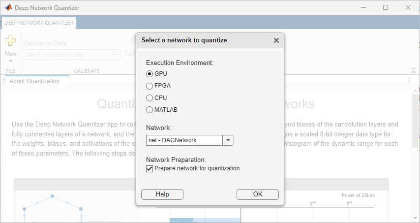
Quantization: Optimize network for quantization with new network preparation step
Prepare your network before calibration by using the new prepareNetwork function or the Network Preparation step in the Deep
Network Quantizer app.
Network preparation modifies your network to improve accuracy and performance, while
also helping to avoid errors during calibration, quantization, and validation. These
modifications include converting your DAGNetwork or
SeriesNetwork objects to dlnetwork
objects.
Quantization: Optimize network for quantization with new network preparation step
Quantization: calibrate supports deep learning arrays
The calibrate
function now supports dlarray objects as calibration data input for
dlnetwork objects.
Functionality being removed or changed
Fixed-Point Designer license required for quantization with MATLAB Execution Environment
Behavior change
When you use the MATLAB Execution Environment for quantization, simulation of the
network is performed using the fi (Fixed-Point Designer) fixed-point data type. This
simulation requires a Fixed-Point Designer™ license for the quantization and validation steps of the deep learning
quantization workflow.
Unconverted DAGNetwork and SeriesNetwork
objects are not supported for quantization with MATLAB Execution Environment
Behavior change
When you use the MATLAB Execution Environment for quantization,
DAGNetwork and SeriesNetwork objects must
be converted to dlnetwork objects before calibration. Use the new
prepareNetwork function or Network Preparation step in the
Deep Network Quantizer app to convert your network to a dlnetwork
object.
DAGNetwork and SeriesNetwork objects are no
longer supported for calibration, quantization, and validation with the MATLAB
Execution Environment.
Interoperability
PyTorch and TensorFlow Importers: Use networkLayer to represent network
composition
Behavior change in future release
When importing a PyTorch® or TensorFlow™ network using the importNetworkFromPyTorch or importNetworkFromTensorFlow functions, you can now specify how the
imported network represents network composition. Use the
PreferredNestingType name-value argument to import a nested
network as a networkLayer
object or a nested custom layer. For more information, see Deep Learning Network Composition.
Starting in R2024b, by default, the importNetworkFromPyTorch and importNetworkFromTensorFlow functions represent network composition
using networkLayer objects. Before 2024b, the functions use nested custom
layers.
PyTorch Import Layer, Operator, and Function Support: Import networks with new layers, operators, and functions
You can now use the importNetworkFromPyTorch function to import the following PyTorch operator and layers into Deep Learning Toolbox layers:
torch.clonetorch.nn.AdaptiveAvgPool2dtorch.nn.Dropout2Dtorch.nn.PReLU
You can also use the importNetworkFromPyTorch
function to import the following PyTorch operators, functions, and layers into custom layers:
torch.abstorch.arangetorch.baddbmmtorch.bitwise_nottorch.costorch.cumsumtorch.getorch.remaindertorch.repeat_interleavetorch.sintorch.rsqrttorch.zeros_liketorch.nn.functional.padtorch.nn.functional.gluandtorch.nn.GLU
PyTorch Importer: Import traced networks from PyTorch 2.0
You can now use the importNetworkFromPyTorch function to import a traced network created
using PyTorch 2.0. Before 2024b, importNetworkFromPyTorch
supported importing networks created using PyTorch versions 1.10.0 and older.
TensorFlow Import Layer and Operator Support: Import networks with new layers and operators
You can now use the importNetworkFromTensorFlow function to import the following TensorFlow layers into Deep Learning Toolbox layers:
tf.keras.layers.Identitytf.keras.layers.LayerNormalizationtf.keras.layers.SpatialDropout1Dtf.keras.layers.SpatialDropout2Dtf.keras.layers.SpatialDropout3D
You can now use the importNetworkFromTensorFlow function to
import the following operators into custom layers:
tf.raw_ops.Erftf.raw_ops.ResourceGather
TensorFlow Export Layer Support: Export networks with four new layers
You can now use the exportNetworkToTensorFlow function to export a Deep Learning Toolbox network that contains the following layers:
ONNX Import Operator Support: Import networks with new operators
You can now use the importNetworkFromONNX function to import the following ONNX™ operators into Deep Learning Toolbox layers:
LayerNormalizationPReluIdentity
You can now use the importNetworkFromONNX function to import the
following ONNX operators into custom layers:
BernoulliGatherNDGridSampleModReduceL1ReduceLogSumReduceLogSumExpReduceSumSquare
ONNX Export Layer Support: Export networks with five new layers
You can now use the exportONNXNetwork function to export a Deep Learning Toolbox network that contains the following layers:
ONNX Version Support: Updated support for ONNX intermediate representation and operator sets
The functions importNetworkFromONNX, importONNXFunction, and exportONNXNetwork now support ONNX intermediate representation version 9
and ONNX operator sets 6 to 18.
Verification
Constrained Deep Learning: Build, train, and verify constrained deep neural networks (GitHub)
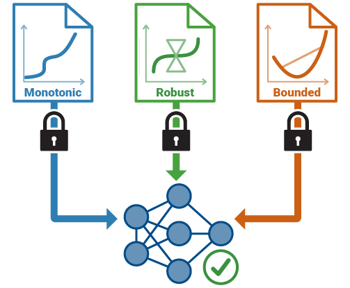
Use the AI Verification: Constrained Deep Learning GitHub repository to build, train, and verify constrained neural networks. Constrained neural networks are networks that adhere to specific constraints, for example, monotonicity. By integrating these constraints into the construction and training of neural networks, you can guarantee desirable behavior and verify the robustness of your network.
You can use this repository to build and train networks that satisfy these constraints:
Monotonicity — Use this property to guarantee that for increasing inputs, the network is either always increasing or always decreasing.
Lipschitz continuity — Use this property to control variation in the network output when inputs are varied. You can use this property to measure robustness.
Convexity — Use this property to guarantee that for a subset of inputs, the network outputs are convex functions. You can use this property to efficiently compute network output bounds.
This repository contains functions to help you build and train constrained networks and uses MATLAB unit tests to verify the behavior of the functions. You can find introductory examples to help you get started as well as longer workflow examples. For example, you can see how to train constrained networks for remaining useful life and neural ODE tasks. For more information about each technique, the repository also contains technical articles that discuss the underlying algorithms. To open all the files in MATLAB Online™, from the GitHub® repository, click Open in MATLAB Online.
Constrained Deep Learning: Build, train, and verify constrained deep neural networks (GitHub)
Formal Methods: Verify branched networks (February 2025; Version 24.2.2)
The verifyNetworkRobustness and
estimateNetworkOutputBounds functions now support networks with
addition layers. You can use addition layers to create branched networks. To add an
addition layer to your network, use the additionLayer function.
Application Examples
Deep Learning Workflows: New and updated examples and topics
Use these new examples and topics to progress with deep learning:
Build Simple App For Deep Learning Inference Using App Designer
Train Network on Amazon Web Services Using MathWorks Cloud Center
Use Experiment Manager in the Cloud with MathWorks Cloud Center
Prepare Data for Battery State of Charge Estimation Using Deep Learning
Train Deep Learning Network for Battery State of Charge Estimation
Compress Deep Learning Network for Battery State of Charge Estimation
Test Deep Learning Network for Battery State of Charge Estimation
Integrate AI Model into Simulink for Battery State of Charge Estimation
Generate Code for Battery State of Charge Estimation Using Deep Learning
Wireless Communications: New examples
Use these new examples for wireless communications tasks:
The Compare Residual Recurrent Neural Network Structures for Digital Predistortion Design example compares residual RNN structures for a digital predistortion (DPD) design.
The CSI Feedback with Transformer Autoencoder example designs and trains a convolutional transformer deep neural network for channel state information feedback by using a downlink clustered delay line (CDL) channel model.
The Model-Free Training of AI-Based OFDM Wireless Systems example uses a custom training loop and loss function for model-free training on an OFDM-based communications system.
The Bluetooth LE Positioning with Deep Learning (Bluetooth Toolbox) example enables you to compute the 3-D position of a Bluetooth® low energy (LE) node by using received signal strength indicator (RSSI) fingerprinting and convolutional neural network (CNN).
Image Processing and Computer Vision: New and updated examples
Use these new and updated examples and topics for image processing and computer vision tasks:
Automatically Label Ground Truth Using Segment Anything Model (Computer Vision Toolbox)
Segment Objects Using Segment Anything Model (SAM) in Image Segmenter (Image Processing Toolbox)
Interactively Segment and Analyze ROI Using MedSAM and Radiomics (Medical Imaging Toolbox)
Segment and Analyze Brain MRI Scan Using AI (Medical Imaging Toolbox)
Detect Small Objects Using Tiled Training of YOLOX Network (Computer Vision Toolbox)
Detect Defects Using Tiled Training of EfficientAD Anomaly Detector (Computer Vision Toolbox)
Signal Processing: New and updated examples
Use these new and updated examples for signal processing tasks:
Real-Time Noise Detection on Raspberry Pi Using Deep Signal Anomaly Detector
Fault Detection and Localization in Three-Phase Power Transmission Using Deep Signal Anomaly Detector in Simulink (DSP System Toolbox)
Musical Instrument Classification with Joint Time-Frequency Scattering
Machine Learning and Deep Learning Classification Using Signal Feature Extraction Objects (Signal Processing Toolbox)
Accelerate Signal Feature Extraction and Classification Using a GPU (Signal Processing Toolbox)
Accelerate Signal Feature Extraction and Classification Using a Parallel Pool of Workers (Signal Processing Toolbox)
Wireless Resource Allocation Using Graph Neural Network (Signal Processing Toolbox)
Denoise Signals with Generative Adversarial Networks (Signal Processing Toolbox)
Speaker Diarization Using Pretrained AI Models (Audio Toolbox)
Train End-to-End Speaker Separation Model (Audio Toolbox)