Ground Truth Labeling
Labeler Enhancements: Edit cuboid ROI labels more easily in top, side, and front 2-D view projections, segment ground from lidar data using SMRF algorithm
The following table describes enhancements for these labeling apps:
Lidar Labeler (Lidar Toolbox)
| Enhancement | Image Labeler | Video Labeler | Ground Truth Labeler | Lidar Labeler |
|---|---|---|---|---|
Show or hide labels and sublabels of type Rectangle,
Line, Polygon, and
Projected cuboid in a labeled image or video. | Yes | Yes | Yes | No |
Show or hide labels of type Cuboid in a labeled point
cloud or point cloud sequence. | No | No | Yes | Yes |
| View and edit cuboid ROI labels using top, side, and front 2-D view projections by selecting Projected View. | No | No | Yes | Yes |
Segment ground from lidar data using the simple morphological filter
(SMRF) algorithm. For more information about the algorithm parameters, see
the segmentGroundSMRF (Lidar Toolbox) function. | No | No | Yes (only with Point Cloud Toolbox™ license) | Yes |
Extract video scenes and corresponding labels from a
groundTruth or
groundTruthMultisignal object. | No | Yes | Yes | No |
| Digital Imaging and Communication in Medicine (DICOM) image format. | Yes | No | No | No |
Velodyne Lidar Sources: Load data from Velodyne VLS-128 lidar device into Ground Truth Labeler app
Load data captured using the Velodyne® VLS-128 lidar device into the Ground Truth Labeler app. Use the vision.labeler.loading.VelodyneLidarSource class to load signals
from the packet capture (PCAP) file data source by setting the
DeviceModel field of the SourceParams
property to "VLS-128".
Cuboid Scenario Simulation
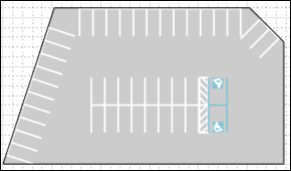
Parking Lots: Add parking lots to driving scenarios programmatically
In drivingScenario objects, use the parkingLot function to create parking lot environments in which
to test your automated driving algorithms. You can choose from a variety of
predefined parking lot layouts or design a custom layout.
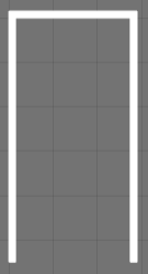
To customize the design of the parking spaces, create parkingSpace objects and visualize them by using the plot function.
To add parking spaces along the edges of parking lots or to add parking grids
at specific positions or orientations, use the insertParkingSpaces function.
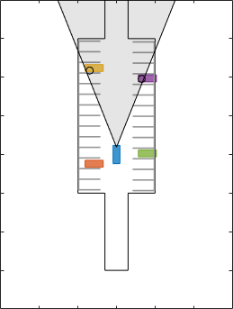
You can also visualize parking lanes on a bird's-eye plot. First, create a
lane marking plotter. Then, obtain the parking lane vertices by using the
parkingLaneMarkingVertices function and plot the lanes by using
the plotParkingLaneMarking function.
For examples that use scenario and sensor simulation in parking lots, see Simulate Vehicle Parking Maneuver in Driving Scenario and Visualize Automated Parking Valet Using Cuboid Simulation.
Note
The creation of parking lots using the Driving Scenario
Designer app is not supported. The import of parking lots into the
app is also not supported. For more details on parking lot limitations, see
the parkingLot reference page.
ASAM OpenDRIVE Import Enhancements: Import a road network using OpenDRIVE file version V1.5 and ASAM OpenDRIVE V1.6
You can now import a road network from OpenDRIVE® file version V1.5 and ASAM OpenDRIVE® V1.6 into a driving scenario by using the roadNetwork function of the drivingScenario object, or by using the Driving Scenario Designer app. In addition, you can now add roads and
export a MATLAB® function after importing the road network into the app.
ASAM OpenDRIVE Export Enhancements: Export a road network to OpenDRIVE file version V1.5 and ASAM OpenDRIVE V1.6
You can now export a driving scenario to OpenDRIVE file version V1.5 and ASAM OpenDRIVE V1.6 by using the Driving Scenario Designer app or the export function of the drivingScenario object.
Use the OpenDRIVEVersion name-value argument of the
export function to specify the version of the file. You can also
specify whether to export actors by using the ExportActors
name-value argument. For
example:
filename = "newfile.xodr";
export(scenario,"OpenDRIVE",filename,OpenDRIVEVersion=1.6,ExportActors=false);
ASAM OpenSCENARIO Export Enhancements: Export the routes of actors using instances
of Trajectory element
When you export a driving scenario to an ASAM OpenSCENARIO® file, the file now specifies the routes of actors using instances
of the Trajectory element. Previously, the routes of actors
were exported separately using a RouteCatalog file containing
instances of the Route element.
Scenario Reader Block: Obtain position, velocity, orientation, and acceleration information from Ego Vehicle State port
The Scenario Reader block now outputs ego vehicle state information that includes the position, velocity and acceleration measurements of the ego vehicle in world coordinates. This information can be used as ground truth data for simulating sensor models, such as an INS sensor. This output is available only in open-loop workflows without ego vehicle pose input to the Scenario Reader block.
INS Block: Generate synthetic readings from an inertial navigation and GPS sensor in driving scenarios in Simulink
Use the INS block to simulate an INS sensor in Simulink®. Obtain the state of the ego vehicle from the Ego Vehicle State output port of the Scenario Reader block. State information includes the position, velocity, orientation, and acceleration of the vehicle. Pass this ego vehicle state information as ground truth to the INS block, which then generates sensor readings at each simulation time step. For an example, see Generate INS Measurements from Driving Scenario in Simulink.
You can now also export scenarios that model INS sensors modeled using the Driving Scenario Designer app to Simulink. For more information, see Generate INS Sensor Measurements from Interactive Driving Scenario.
Road Heading Angles: Create more precise roads using fewer road centers
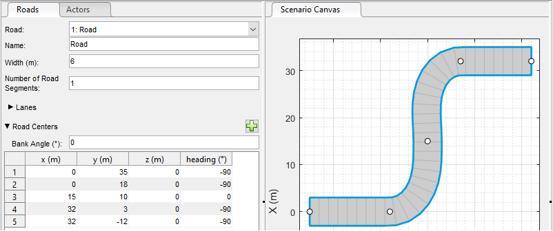
You can now specify heading angles at road centers to create roads. Specifying heading angles as a constraint to road center points enables finer control over the shape and orientation of roads using fewer road centers.
To programmatically add roads with heading angles to a drivingScenario object, use the Heading
name-value argument of the road function. Specify the heading value as a column vector of
angles in the range [–180, 180] degrees. For
example:
road(scenario,roadCenters,Heading=[-90;-90;0;-90;-90]);
This figure shows two roads with the same road centers, but one has specified heading angle values and the other does not.
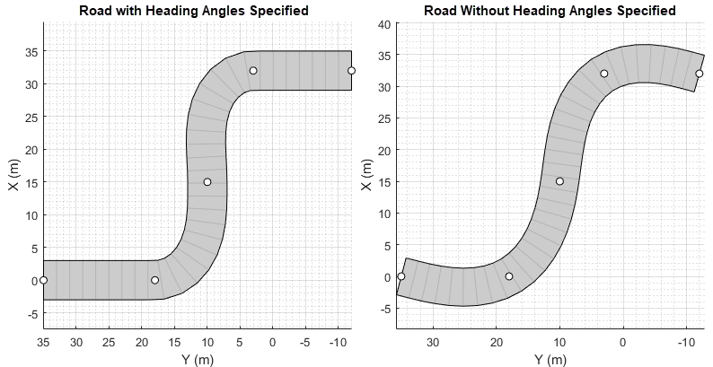
You can also use the Driving Scenario Designer app to specify road heading angles. Use the heading column in the Road Centers table to specify the heading angles at each road center.
Lane Generation Example: Add lane information to map imported road network
The Generate Lane Information from Recorded Data example shows how to generate lane information using recorded data from a camera and a GPS sensor. Use this example to add lane information to a road network imported from SD map data.
Scenario Generation Examples: Generate scenario from recorded sensor data and scenario variants from seed scenario
The Generate Scenario from Recorded GPS and Lidar Data example shows how to automatically generate a driving scenario from the data recorded by global positioning systems (GPS) and lidar sensors. You can use the generated scenario as input data to model and simulate an automated driving system.
The Automatic Scenario Variant Generation for Testing AEB Systems example shows how to automatically generate variants of a seed scenario in which two actors collide. You can generate random variants of a collision scenario and use them to design and validate an automated emergency braking (AEB) system.
Unreal Engine Scenario Simulation
Unreal Engine Environment Upgrade: Run 3D simulations using Unreal Engine, Version 4.25
The 3D simulation engine that comes installed with Automated Driving Toolbox™ has been updated to Unreal Engine®, Version 4.25. Previously, the toolbox used Unreal Engine, Version 4.23.
For information about using Unreal Engine to create custom scenes, see Customize Unreal Engine Scenes for Automated Driving.
If your Simulink model uses an Unreal Engine executable or project developed using a prior release of the Automated Driving Toolbox Interface for Unreal Engine Projects support package, the simulation might produce an error. To migrate the project so that it is compatible with the R2021b version of the support package, see Migrate Projects Developed Using Prior Support Packages.
Position Adjustments of Unreal Engine Cameras: Update relative translation and rotation of camera sensors during simulation
In the Simulation 3D Camera and Simulation 3D Fisheye Camera blocks, use the Translation and Rotation input ports to update the position of the cameras relative to their mounting positions during simulation. You can use these position adjustments to better model actuator dynamics, isolation mounting, and calibration workflows.
Previously, you could set only constant relative positions by using the Relative translation [X, Y, Z] (m) and Relative rotation [Roll, Pitch, Yaw] (deg) parameters. Now, by selecting Input to enable the corresponding ports, the parameters specify the initial position and the ports specify the position during simulation.
Unreal Engine Environment Performance Improvements: Run 3D simulations faster than real-time
Simulink co-simulations with Unreal Engine can now run faster than real-time. Previously, the Unreal Engine frame rate was limited by the inverse of the simulation sample rate. If you want to slow down a 3D simulation to investigate system behavior, you can still use simulation pacing.
Use the Simulation 3D Scene Configuration block parameter Sample time to control simulation time. For example,
if Sample time is 1/30,
then the visualization engine solver tries to achieve a minimum frame rate of 30
frames per second (FPS). However, the real-time graphics frame rate is often
lower due to factors such as graphics card performance and model complexity.
With sufficient graphics card performance and low model complexity, the frame
rate could be greater than 30 FPS, not limited to 30 FPS as in previous
releases.
Unreal Engine Visualization Example: Visualize logged data for post-simulation analysis
The Visualize Logged Data from Unreal Engine Simulation example shows how to customize the visualization of logged sensor and simulation data using the Simulation Data Inspector. This example enables you to analyze and debug automated driving test cases after running the simulation.
Detection and Tracking
Perturbations: Perturb object properties using truncated normal distribution
You can now define the perturbation distribution of a property as a truncated
normal distribution using the perturbations (Sensor Fusion and Tracking Toolbox) function.
With offset values bounded by a finite interval, the truncated normal
distribution is suitable for perturbing a property whose valid values are
confined in a finite interval.
Code Generation: Generate more memory-efficient C/C++ code from trackers and tracking filters
These objects and Simulink blocks now support strict single-precision and static memory allocation code generation:
See the Extended Capabilities section on each object or block reference page for its code generation limitations.
Radar and Tracking Examples: Fuse radar and camera tracks, track using event-based sensor fusion and retrodiction and track in scenarios with multipath radar reflections in Simulink
The Extended Object Tracking of Highway Vehicles with Radar and Camera in Simulink example shows how to fuse radar and camera measurements to track highway vehicles with multiple extended object tracking techniques and evaluate their tracking performance in Simulink. This example requires the Sensor Fusion and Tracking Toolbox™ software.
The Event-Based Sensor Fusion and Tracking with Retrodiction example shows how to track vehicles using event-based sensor fusion of simulated radar and camera measurements in Simulink. This example requires the Sensor Fusion and Tracking Toolbox software.
The Extended Target Tracking with Multipath Radar Reflections in Simulink example shows how to model and mitigate multipath radar reflections during highway vehicle tracking in Simulink. This example requires the Sensor Fusion and Tracking Toolbox. It closely follows the Highway Vehicle Tracking with Multipath Radar Reflections (Radar Toolbox) example.
Track moving vehicles with multiple lidar sensors using a grid-based tracker in Simulink
The Grid-based Tracking in Urban Environments Using Multiple Lidars in Simulink example shows how to track moving vehicles in urban environments with measurements from multiple lidar sensors using a grid-based tracker in Simulink. This example requires the Sensor Fusion and Tracking Toolbox software. It closely follows the Grid-Based Tracking in Urban Environments Using Multiple Lidars example.
Perform dynamic replanning on highways using tracking in MATLAB
The Object Tracking and Motion Planning Using Frenet Reference Path example shows how to perform dynamic replanning on highways using a Frenet reference path and a joint probabilistic data association (JPDA) tracker in MATLAB. This example requires the Sensor Fusion and Tracking Toolbox and Navigation Toolbox™ software. It is an extension of the Highway Trajectory Planning Using Frenet Reference Path example.
Localization and Mapping
Visual Localization Example: Develop and evaluate a visual localization algorithm in a parking lot scenario
The Visual Localization in a Parking Lot example shows how to develop a visual localization system using synthetic image data from the Unreal Engine simulation environment.
Segment Matching Example: Build Map and Localize Using Segment Matching
The Build Map and Localize Using Segment Matching example shows how to build a map with lidar data and localize the position of a vehicle on the map using SegMatch, a place recognition algorithm based on segment matching.
Applications
Message-Based Communication: Establish message-based communication between model components
The Generate C++ Message Interfaces for Lane Following Controls and Sensor Fusion example shows how to establish message-based communication between the controller and sensor fusion components of a highway lane following system. This workflow enables you to integrate system components in a distributed architecture.
Real-Time Testing: Deploy and test highway lane following controller in real-time
The Automate Real-Time Testing for Highway Lane Following Controller example shows how to configure a hardware setup to deploy a lane following controller to a Speedgoat® real-time machine. The example also shows how to automate the regression testing of the deployed application.
Automate Testing: Automate testing of components of lane following and lane changing systems
These new examples show how to automate testing and verify generated code for different components of highway lane following and highway lane change systems.