R2022a

New Features, Bug Fixes, Compatibility Considerations

Ground Truth Labeling

Labeler Enhancements: 3D line ROI labels for point clouds

The following table describes enhancements for these labeling apps:

EnhancementImage Labeler Video Labeler Ground Truth Labeler Lidar Labeler
Draw, visualize, and export semantic labels in the point cloud.NoNoNoYes
Create training data for object detection in point clouds by using the lidarObjectDetectorTrainingData function.NoNoNoYes
Import multiframe DICOM images.YesNoNoNo
Create 3-D line ROI for point cloud data.NoNoYesYes
Create voxel ROI for point cloud data.NoNoNoYes
Show or hide pixel labels in a labeled image or video.YesYesYesNo

File I/O

 ADTF File Reader: Read data from Automotive Data and Time-Triggered Framework (ADTF) DAT file

Automated Driving Toolbox™ now supports reading data from files stored in the Automated Data and Time-Triggered Framework (ADTF), developed by Elektrobit for automated driving applications. Use the adtfFileReader object to read stream information and inspect the contents of an ADTF DAT file. To select the messages of a specific sensor from this file, use the select function. You can then use the read or readNext function to read the messages contained in the file, and use these messages in automated driving workflows. For an example, see Read Data From ADTF DAT Files.

Reading ADTF DAT files is not supported for Mac platforms.

Cuboid Scenario Simulation

Ultrasonic Sensor Model: Generate synthetic range measurements from programmatic driving scenarios and Driving Scenario Designer app

Use the ultrasonicDetectionGenerator System object™ to model an ultrasonic sensor and generate synthetic range data for actors in a drivingScenario object. To visualize the ultrasonic detections on a bird's-eye plot, create a rangeDetectionPlotter object, and then plot the set of ranges using the plotRangeDetection function.

In the Driving Scenario Designer (DSD) app, you can now model an ultrasonic sensor and generate synthetic range data from a driving scenario. The bird's-eye-plot in the DSD app visualizes the ranges detected by the ultrasonic sensor as arcs. When you export a scenario containing an ultrasonic sensor to MATLAB®, the sensor is represented as an ultrasonicDetectionGenerator System object.

Bird's-Eye Scope Enhancement: Run simulations from previously saved models without finding signals again

When visualizing signals in Simulink® models by using the Bird's-Eye Scope, you can now immediately visualize signals logged from the last time you saved and closed the model. Previously, when reopening a model, you had to click Find Signals to find all signals in the model again before visualizing them. To find and visualize new signals in a reopened model, click Update Signals.

Radar Sensor Performance Enhancement: Simulate driving scenarios with radar sensors faster in MATLAB and Simulink

Radar sensors modeled using drivingRadarDataGenerator system object or Driving Radar Data Generator block now have improved simulation performance in complex driving scenarios with extended targets. For a driving scenario containing 7 radar sensors, a 42% average performance improvement has been observed on Windows 10 platform.

ASAM OpenSCENARIO Export Enhancements: Export road networks, actors, and trajectories to ASAM OpenSCENARIO file version 1.1

You can now export a driving scenario to ASAM OpenSCENARIO® file version 1.1 by using the Driving Scenario Designer app or the export function of the drivingScenario object.

Use the OpenSCENARIOVersion name-value argument of the export function to specify the version for the file. For example:

filename = "newfile.xosc";
export(scenario,"OpenSCENARIO",filename,OpenSCENARIOVersion=1.1);

Sharp Curvature Roads: Create or import roads with sharp curvature

You can now create or import roads with sharp curvature using the road function or roadNetwork function, respectively, of the drivingScenario object. Previously, creating or importing sharp curvature roads was not supported.

You can also interactively create or import roads with sharp curvature using the Driving Scenario Designer app.

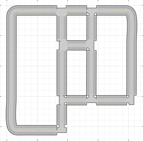
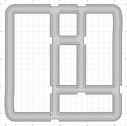
This table shows an example of enhanced ASAM OpenDRIVE® road network imported using R2022a compared to the road network imported using R2021b.

R2021bR2022a

A road network imported from ASAM OpenDRIVE file using R2021b. The imported network ignores the bottom-right road with sharp curvature.

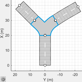
A road network imported from ASAM OpenDRIVE file using R2022a. The imported network includes the bottom-right road with sharp curvature.

Road Group Enhancements: Import heading angle information of road groups into the Driving Scenario Designer app

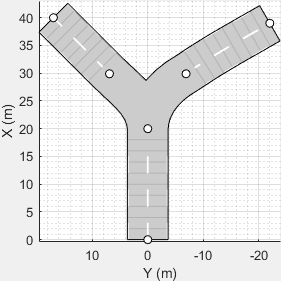
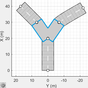
When you import a drivingScenario object into the Driving Scenario Designer app, you can now import heading angles of road segments stored within the RoadGroup object. Previously, heading angle information of road groups was not imported into the app. In addition, you can also export the heading angle information of road groups to a MATLAB function from the app. This heading angle information enables you to accurately match the shapes of road groups across programmatic and interactive workflows as shown in this figure.

Scenario created using drivingScenario objectScenario imported in the app using R2021bScenario imported in the app using R2022a

Road network created using drivingScenario object. This road network contains a road group.

Road network after importing drivingScenario object into the app using R2021b.

Road network after importing drivingScenario object into the app using R2022a.

Ego Localization Example: Correct ego vehicle localization using recorded sensor data

The Improve Ego Vehicle Localization example shows how to correct ego vehicle localization and generate an accurate ego trajectory by fusing global positioning system (GPS) and inertial measurement unit (IMU) sensor data. The example also shows how to compose a virtual driving scenario using a localized ego trajectory and OpenStreetMap® road network.

Unreal Engine Scenario Simulation

Simulation 3D Lidar Reflectivity: Model surface reflections in Unreal Engine environment

In the Simulation 3D Lidar block, use the Reflectivity output port to output the reflectivity of surface materials in the Unreal Engine® environment.

OpenCV Radial Distortion in Simulation 3D Camera Block: Simulate cameras with OpenCV supported radial distortion model in Unreal Engine Environment

In the Simulation 3D Camera block, you can now use the OpenCV six-coefficient formula for modeling radial distortion. Specify the formula to the Radial distortion coefficients parameter. This is in addition to the two-coefficient and three-coefficient models already supported by camera calibration tools in Computer Vision Toolbox™. For more information on calibrating a camera using the six-coefficient formula, see Camera Calibration and 3D Reconstruction in the OpenCV documentation.

Simulation 3D Camera Performance Improvements: Run cameras at improved speeds during Unreal Engine simulation

The Simulation 3D Camera block now has improved simulation performance and runs at higher frame rates. This table shows the increase in frames per second (FPS) for each camera in an Unreal Engine simulation.

Number of Cameras in SimulationFrame Rate per Camera (R2021b)Frame Rate per Camera (R2022a)Percent Improvement per Camera
175.85 FPS88.45 FPS16.6%
430.51 FPS32.80 FPS7.5%

These simulations were timed on a Windows 10, Intel® Xeon® W-2133 CPU @ 3.60 GHz, with 64 GB of RAM and a GPU with 8 GB of on-board RAM.

These improvements enable you to run cameras at real-time speeds, provided that your system meets the requirements specified by the Unreal Engine Simulation Environment Requirements and Limitations.

 Simulation 3D Environment Upgrade: Run 3D simulations using Unreal Engine 4.26

The 3D visualization engine that comes installed with Automated Driving Toolbox has been updated to Unreal Engine 4.26. Previously, the toolbox used Unreal Engine 4.25.

For information about using Unreal Engine to create custom scenes, see Customize Unreal Engine Scenes for Automated Driving and Unreal Engine Simulation Environment Requirements and Limitations.

 Compatibility Considerations

If your Simulink model uses an Unreal Engine executable or project developed using a prior release of the Automated Driving Toolbox Interface for Unreal Engine Projects support package, the simulation may return an error. To migrate the project so that it is compatible with the R2022a version of the support package, see Migrate Projects Developed Using Prior Support Packages.

 Functionality being removed or changed

Updated Large Parking Lot scene

Behavior change

Starting from R2022a, the Large Parking Lot scene in the Unreal Engine 3D environment is rendered using RoadRunner. As a result, the locations of scene objects, including cones and parked vehicles, are moved from their pre-R2022a locations.

RoadRunner Scenario Simulation

Simulate RoadRunner scenarios with MATLAB and Simulink

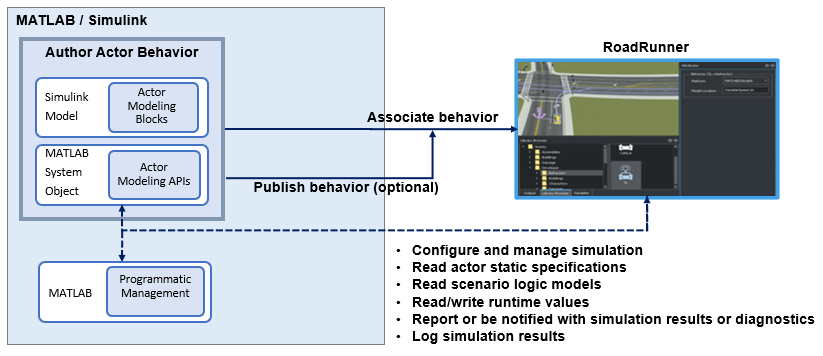
RoadRunner is an editor that enables you to design 3D scenes for simulating and testing automated driving systems. In R2022a, Automated Driving Toolbox provides a cosimulation framework for simulating scenarios in RoadRunner with actors modeled in MATLAB and Simulink.

These are the steps of the simulation workflow:

Overview of the MATLAB or Simulink and RoadRunner scenario cosimulation workflow

Use these new objects to view and control the attributes of a RoadRunner scenario simulation and its associated actors through MATLAB:

You can use these objects and functions in MATLAB System Objects to create custom RoadRunner actor behaviors.

Use these new blocks to create a model to define custom behaviors for your actors in RoadRunner using Simulink:

Explore these examples that demonstrate speed action follower, trajectory follower, and highway lane change planner workflows with RoadRunner Scenario cosimulation:

  • The Speed Action Follower with RoadRunner Scenario example shows how to design speed action following behavior using MATLAB. You assign this behavior to the ego vehicle in the RoadRunner scenario and control the speed of the ego vehicle to avoid collision with a lead car. The example also shows how to visualize RoadRunner Scenario simulation data using MATLAB.

  • The Trajectory Follower with RoadRunner Scenario example shows how to control the motion of the ego vehicle in RoadRunner Scenario using Simulink to follow the specified trajectory. The example uses the Stanley controller and 3DOF vehicle dynamics to control the motion of the ego vehicle. The example also shows how to visualize RoadRunner Scenario simulation data using MATLAB.

  • The Highway Lane Change Planner with RoadRunner Scenario example shows how to simulate a lane change behavior for the ego vehicle in a RoadRunner scenario by using Simulink. The example uses a highway lane change planner Simulink model that finds an optimal collision-free trajectory to navigate the ego vehicle.

These examples require licenses for RoadRunner and RoadRunner Scenario.

MATLAB Functions for RoadRunner Scenes and Scenarios: Import and export RoadRunner scenes and scenarios programmatically

Using the roadrunner object and its associated MATLAB functions, you can control the RoadRunner application programmatically. Common programmatic tasks that you can perform include:

  • Open and close the RoadRunner application.

  • Open, close, and save scenes and projects.

  • Import and export scenes.

These MATLAB functions require an Automated Driving Toolbox license. For details on using these functions, see MATLAB Functions for Scenes (RoadRunner) and MATLAB Functions for Scenarios (RoadRunner Scenario).

Detection and Tracking

YOLO v4 Object Detection: Detect objects in monocular camera images using you only look once version 4 (YOLO v4) deep learning network

The configureDetectorMonoCamera function can now configure a monocular camera to use the YOLO v4 object detector, returning an yolov4ObjectDetectorMonoCamera object.

Bird's-Eye View Example Update: Generate code for algorithm to create 360° bird's-eye-view image around a vehicle

The Create 360° Bird's-Eye-View Image Around a Vehicle example now shows how to generate code for algorithm to create 360° bird's-eye-view image around a vehicle for use in a surround-view monitoring system. It also shows how to verify the generated code before deployment.

PIL Verification of JPDA Tracker Example: Generate embedded code and perform processor-in-loop (PIL) verification of JPDA tracker in highway scenarios

The Processor-in-the-Loop Verification of JPDA Tracker for Automotive Applications example shows how to generate embedded code for a joint probabilistic data association (JPDA) tracker configured to process detections from a camera and radar sensor mounted on the front of the ego vehicle in highway scenarios. It also shows how to verify the generated code using processor-in-loop (PIL) simulation on an STM32 Nucleo board using simulated detections.

 Functionality being removed or changed

Bug fixes and behavior changes of trackingKF object

Behavior change

As of R2022a the trackingKF filter object has these behavior changes:

  • If you set the MotionModel property to a predefined state transition model, such as "1D Constant Velocity", you can no longer specify the control model for the filter. To use a control model, specify the MotionModel property as "Custom".

  • You must now specify the control model of the filter when creating the filter. You can no longer specify it after creating the filter.

  • You can now specify the process noise for a trackingKF object using the ProcessNoise property for a predefined motion model. The dimension of the process noise matrix set through the ProcessNoise property now differentiates between a predefined motion model and a customized motion model. Specifically,

    • If the specified motion model is a predefined motion model, specify the ProcessNoise property as a D-by-D matrix, where D is the dimension of the motion. For example, D = 2 for "2D Constant Velocity" motion model.

    • If the specified motion model is a customized motion model, specify the ProcessNoise property as an N-by-N matrix, where N is the dimension of the state. For example, N = 4 if you customize a 2-D motion model in which the state is (x, vx, y, vy).

  • The orientation of the filter state now matches the state vector that you specify when creating the filter. For example, if you set the initial state in the filter as a row vector, the filter displays the filter state as a row vector. Previously, the filter displayed the filter state as a column vector regardless of initial state.

  • You can generate efficient C/C++ code without dynamic memory allocation for trackingKF.

Localization and Mapping

Parking Spot Detection Example: Detect empty parking spots in a parking lot using semantic segmentation

The Perception-Based Parking Spot Detection Using Unreal Engine Simulation example shows how to detect lane markings and obstacles in a parking lot using semantically segmented camera images, incrementally update detections in the bird’s-eye view, reconstruct parking spots from lane markings, and build a map of parking spots for decision making in an Unreal Engine simulation environment.

LOAM Example: Build map and localize using Lidar Odometry and Mapping (LOAM)

The Build a Map with Lidar Odometry and Mapping (LOAM) Using Unreal Engine Simulation example shows how to build a map with lidar data and localize the position of a vehicle on the map using Lidar Odometry and Mapping (LOAM), an algorithm that uses edge and surface points in the point cloud for registration and mapping.

Point Cloud Localization Example Update: Localize with a prebuilt map using NDT algorithm

The Lidar Localization with Unreal Engine Simulation example now shows how to localize the position of a vehicle on a prebuilt map using the Normal Distributions Transform (NDT) algorithm.

Visual SLAM Example Update: Reconstruct a parking lot from stereo images using visual SLAM

The Develop Visual SLAM Algorithm Using Unreal Engine Simulation example now shows how to perform dense reconstruction using stereo images of a parking lot scene in an Unreal Engine simulation environment.

Applications

Intersection Navigation Examples: Use V2V and V2X communication technologies to build applications for safe navigation through intersections

The Intersection Movement Assist Using Vehicle-to-Vehicle Communication example shows how to design and test an intersection movement assist (IMA) application by modeling vehicle-to-vehicle (V2V) communication. In this example, you also study the effect of channel impairments on the IMA application.

The Traffic Light Negotiation Using Vehicle-to-Everything Communication example shows how to design and test decision logic using vehicle-to-everything (V2X) communication to negotiate a traffic light to prevent collisions at intersections. This example uses the vehicle-to-vehicle (V2V) and vehicle-to-infrastructure (V2I) modes of V2X communication.

Autonomous Emergency Braking Examples: Integrate high fidelity vehicle dynamics model with autonomous emergency braking (AEB) system and automate testing of AEB system

The Autonomous Emergency Braking with Vehicle Variants example enables you to integrate either 3DOF or 14DOF vehicle models with AEB system in a closed-loop environment. Using this example, you can study interactions between an AEB controller and vehicle dynamics model, and analyze the impact of high-fidelity vehicle dynamics on AEB applications.

The Autonomous Emergency Braking with Sensor Fusion example has been updated to calculate the steering angle required for an ego vehicle to follow the reference path. This capability enables you to test and validate an AEB system using complex Euro NCAP® test scenarios that contain intersections.

The Automate Testing for Autonomous Emergency Braking example shows how to automate testing of the components of an AEB system and verify the generated code using Simulink Test™ software. You can automate testing of the sensor fusion and tracking, decision logic, and controller components.

Real-Time Testing Example: Deploy and test forward vehicle sensor fusion component in real-time

The Automate Real-Time Testing for Forward Vehicle Sensor Fusion example shows how to deploy a forward vehicle sensor fusion component of a highway lane following system to a Speedgoat® real-time machine and automate the regression testing of the deployed application.

Highway Lane Change Example Update: Integrate surround vehicle sensor fusion with highway lane change system

The Highway Lane Change example now integrates a surround vehicle sensor fusion component that provides a 360-degree view for detecting target vehicles surrounding the ego vehicle, enabling it to perform a lane change maneuver. Before R2022a, the example instead used the ground truth information of target vehicles to perform a lane change maneuver for the ego vehicle, as shown in the Highway Lane Change Planner and Controller example.