IF Subsampling with Complex Multirate Filters
This example shows how to use complex multirate filters in the implementation of Digital Down-Converters (DDC). The DDC is a key component of digital radios. It performs the frequency translation necessary to convert the high input sample rates typically found at the output of an analog-to-digital (A/D) converter down to lower sample rates for further and easier processing. In this example, we will see how an audio signal modulated with a 450 kHz carrier frequency can be brought down to a 20 kHz sampling frequency. After a brief review of the conventional DDC architecture, we will describe an alternative solution known as Intermediate Frequency (IF) subsampling and we will compare the respective implementation cost of these two solutions. This example requires a Fixed-Point Designer™ license.
Conventional Digital Down Converter
A conventional down conversion process starts with sampling the analog signal at a rate that satisfies the Nyquist criterion for the carrier. A possible option would be to sample the 450 kHz input signal at 2.0 MHz, then using a digital down converter to perform complex translation to baseband, filter and down sample by 25 with a Cascaded Integrator-Comb (CIC) filter, and then down sample by 4 with a pair of half band filters. Such an implementation is shown below:

CIC Filter Design
The first filter of the conventional DDC is usually a CIC filter. CIC filters are efficient, multiplier-less structures which can be used in decimator and interpolator systems with high conversion ratios. In this case, a CIC decimator with a decimation factor of R = 25 brings the 2 MHz signal down to 2.0 MHz/25 = 80 kHz. For this design, choose the number of sections to be N = 4.
Fs_normDDC = 2e6;  % Sampling frequency
R          = 25;   % Decimation factor
D          = 1;    % Differential delay
Nsecs      = 4;    % Number of sections
cic     = dsp.CICDecimator(R,D,Nsecs);
cicgain = dsp.FIRFilter(Numerator=1/gain(cic)); % Normalize gain of CIC
Compensation FIR Decimator Design
The second filter of the conventional DDC compensates for the passband droop caused by the CIC. Since the CIC has a sinc-like response, it can be compensated for the droop with a lowpass filter that has an inverse-sinc response in the passband.
Fpass = 10e3;             % Passband Frequency
Fstop = 25e3;             % Stopband Frequency
Apass = 0.01;             % Passband Ripple (dB)
Astop = 80;               % Stopband Attenuation (dB)
cfir  = dsp.CICCompensationDecimator(cic,PassbandFrequency=Fpass,StopbandFrequency=Fstop,SampleRate=Fs_normDDC/R,...
                        PassbandRipple=Apass,StopbandAttenuation=Astop);
Halfband Filter Design
We finally use a 20th order halfband filter to bring the 40 kHz signal down to 20 kHz.
hbfilter = designHalfbandFIR(FilterOrder=20,TransitionWidth=0.35,Structure='decim',SystemObject=true);
The conventional DDC filter is obtained by cascading the three stages previously designed.
normDDCFilter = cascade(cicgain,cic,cfir,hbfilter);
IF Subsampling
Since the carrier frequency is discarded as part of the signal extraction, there is no need to preserve it during the data-sampling process. The Nyquist criterion for the carrier can actually be violated as long as Nyquist criterion for the bandwidth of complex envelope is satisfied.
This narrowband interpretation of the Nyquist criterion leads to an alternate data collection process known as IF subsampling. In this process, the A/D converter's sample rate is selected to be less than the signal's center frequency to intentionally alias the center frequency. Since Nyquist criterion is being intentionally violated, the analog signal must be conditioned to prevent multiple frequency intervals from aliasing to the same frequency location as the desired signal component will alias.
The variable y represents approximately 3 sec of an audio signal modulated with a 450 kHz carrier frequency. The discrete signal ys represents the output of a 120 kHz A/D converter.
[y,ys,Fs] = loadadcio;
Fs_altDDC = 1.2e5;   % Sampling frequency

% Calculate aliased A/D output power
[Hys,Fys] = periodogram(ys,[],[],Fs,'power','centered');
N = length(Fys);
F_ADout = ((0:N*R-1)-N*R/2+1)/N*Fs_altDDC/1e3; % kHz units
H_ADout = repmat(Hys,R,1);

figure(color='white')
periodogram(y,[],[],Fs,'power','centered');
clear y
hold on
plot(F_ADout,db(H_ADout)/2,'r:');
axis([-50 500 -160 0])
legend('Input of A/D Converter','Aliased Output of A/D Converter', ...
    Location='NorthEast');
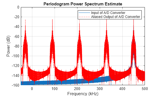
The frequency band around 450 kHz aliased around -30 kHz. Aliasing to a quarter of the sampling frequency maximizes the separation between positive and negative frequency aliases. This permits maximum transition bandwidth for the analog bandpass filter and therefore minimize its cost.
The choice of a 120 kHz sampling frequency also eases the subsequent task of down converting to 20 kHz which is accomplished by down sampling by a factor of 6. The down conversion can be achieved in two stages. First a 3-to-1 downsampling is performed by a complex bandpass filter followed by a 2-to-1 conversion with a half band filter. The structure of this aliasing DDC is shown below.

Complex Bandpass Filter Design
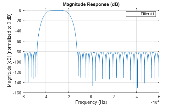
To obtain a complex bandpass filter, we translate a lowpass decimator prototype to quarter sample rate by multiplying the filter coefficients with the heterodyne terms exp(-j*pi/2*n). Notice that while the coefficients of the lowpass filter are real, the coefficients of the translated filter are complex. The figure below depicts the magnitude responses of these filters.
M  = 3;            % Decimation Factor
TW = Fstop-Fpass;  % Transition Width (Hz)
lpfilter = designMultirateFIR(DecimationFactor=3,TransitionWidth=TW,StopbandAttenuation=Astop,InputSampleRate=Fs_altDDC,SystemObject=true);

n = 0:length(lpfilter.Numerator)-1;
complexBPFilter = dsp.FIRDecimator(M,lpfilter.Numerator.*exp(-1i*pi/2*n));

FA = filterAnalyzer(lpfilter.Numerator,1,complexBPFilter,SampleRates=Fs_altDDC,FrequencyRange='centered');
setLegendStrings(FA,["Lowpass Decimator","Complex Bandpass Decimator"])

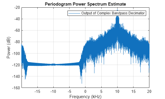
We now apply the complex bandpass decimator to the output of A/D converter. It can be shown that a signal at a quarter sample-rate will always alias to a multiple of the quarter sample-rate under decimation by any integer factor. In our example the -30 kHz centered signal will alias to 40/4 = 10 kHz.
ycbp = complexBPFilter(ys);
figure(color='white')
periodogram(ycbp,[],[],Fs_altDDC/M,'power','centered');
legend('Output of Complex Bandpass Decimator')
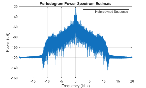
The output sequence ycbp is then heterodyned to zero.
yht = ycbp.*(-1i).^(0:length(ycbp)-1).';
figure(color='white')
periodogram(yht,[],[],Fs_altDDC/M,'power','centered');
legend('Heterodyned Sequence')
Finally the heterodyned sequence is passed as input to the half band filter and decimated by 2. We can reuse the same halfband filter as in the conventional DDC.
yf = hbfilter(yht);
figure(color='white')
periodogram(yf,[],[],Fs_altDDC/(2*M),'power','centered');
legend('Output of Aliasing DDC')

Play the audio signal at the output of the "aliasing" DDC. (Copyright 2002 FingerBomb)
player = audioDeviceWriter(SampleRate=Fs_altDDC/(2*M));
player(real(yf));
Implementation Cost Comparison
Before we proceed to the cost analysis let's verify that the magnitude responses of the filters in the two DDC solutions are comparable. We exclude both the complex translation to baseband in the conventional DDC case and the heterodyne in the IF subsampling case. Furthermore, we use the lowpass prototype decimator in the later case since it has the same transition width, passband ripples and stopband attenuation as the complex band pass decimator.
altDDCFilter = cascade(lpfilter,hbfilter);
We verify that the filters used in both cases have very similar magnitude responses: less that 0.04 dB passband ripple, a 6dB cutoff frequency of 10 kHz and a 55 dB stopband attenuation at 13.4 kHz. It is therefore fair to proceed to the cost analysis.
FA = filterAnalyzer(normDDCFilter,altDDCFilter,SampleRates=[Fs_normDDC,Fs_altDDC],ReferenceFilter=false);
setLegendStrings(FA,["Conventional DDC Filter","Equivalent Digital IF Subsampling Filter"], ...
    FilterNames=["normDDCFilter","altDDCFilter"]);
showFilters(FA,false, ...
    FilterNames=["normDDCFilter_Stage1","normDDCFilter_Stage2","normDDCFilter_Stage3","normDDCFilter_Stage4",...
        "altDDCFilter_Stage1","altDDCFilter_Stage2"]);
zoom(FA,'x',[0 100e3])

In the case of the conventional DDC, we must first take into account the cost of the baseband translation. We are assuming it is done with only one multiplier working at 2 MHz. We must then add the cost of the CIC and halfband filters. In the IF subsampling case, we must consider the cost of the heterodyne. We are assuming it is done with only one multiplier working at 40 kHz. We must then add the cost of the complex bandpass and halfband filters.
% Cost of CIC and halfband filters
c_normDDC = cost(normDDCFilter);
% Cost of complex bandpass and halfband filters
c_altDDC  = cost(cascade(complexBPFilter,hbfilter));
ddccostcomp(Fs_normDDC,c_normDDC,Fs_altDDC,c_altDDC)
ans =
    'Total Cost                      : Conventional DDC | IF subsampling
     -------------------------------------------------------------------
     Number of Coefficients          :               35 |             42
     Number of States                :               50 |             62
     Multiplications per microsecond :             5.14 |            1.5
     Additions per microsecond       :             9.4 |            1.4'
The number of multipliers, adders and states required in the IF subsampling case is comparable to that of conventional DDC but the number of operations per second is significantly reduced since it saves 71% of the number of multiplications per second and 85% of the number of additions per second.
Using dsp.ComplexBandpassDecimator
We can design the complex bandpass filter more easily by using the dsp.ComplexBandpassDecimator System object. The object designs the bandpass filter based on the specified decimation factor, center frequency, and sample rate. There is no need to translate lowpass coefficients to bandpass as we did in the design above: the object will do it for us. Moreover, the object will derive the frequency to which the filtered signal is aliased, and mix it back to zero Hz for us.
% Design a complex bandpass filter. Include the decimate-by-2 halfband
% filter into the design by specifying a decimation factor of 2*M:
bp = dsp.ComplexBandpassDecimator(M*2,-30e3,Fs_altDDC,TransitionWidth=TW);
% Visualize the filter response
visualize(bp);
% Filter the output of the 120 kHz A/D converter
yf = bp(ys);
figure(color='white')
periodogram(yf,[],[],Fs_altDDC/(2*M),'power','centered');
legend('Output of complex bandpass decimator')

player(real(yf));
Summary
This example showed how complex multirate filters can be used when designing IF subsampling-based digital down converters. The IF subsampling technique can be cost efficient alternative to conventional DDCs in many applications. For more information on IF subsampling see Multirate Signal Processing for Communication Systems by fredric j harris, Prentice Hall, 2004.