Vary Mutation and Crossover

Setting the Amount of Mutation

The genetic algorithm applies mutations using the MutationFcn option. The default mutation option, @mutationgaussian, adds a random number, or mutation, chosen from a Gaussian distribution, to each entry of the parent vector. Typically, the amount of mutation, which is proportional to the standard deviation of the distribution, decreases at each new generation. You can control the average amount of mutation that the algorithm applies to a parent in each generation through the Scale and Shrink inputs that you include in a cell array:

options = optimoptions('ga',...
    'MutationFcn',{@mutationgaussian Scale Shrink});

Scale and Shrink are scalars with default values 1 each.

Scale controls the standard deviation of the mutation at the first generation. This value is Scale multiplied by the range of the initial population, which you specify by the InitialPopulationRange option.
Shrink controls the rate at which the average amount of mutation decreases. The standard deviation decreases linearly so that its final value equals 1 – Shrink times its initial value at the first generation. For example, if Shrink has the default value of 1, then the amount of mutation decreases to 0 at the final step.

You can see the effect of mutation by selecting the plot functions @gaplotdistance and @gaplotrange, and then running the genetic algorithm on a problem such as the one described in Minimize Rastrigin's Function. The following figure shows the plot after setting the random number generator.

rng default % For reproducibility
options = optimoptions('ga','PlotFcn',{@gaplotdistance,@gaplotrange},...
    'MaxStallGenerations',200); % to get a long run
[x,fval] = ga(@rastriginsfcn,2,[],[],[],[],[],[],[],options);

Optimization terminated: maximum number of generations exceeded.

Figure Genetic Algorithm contains 2 axes objects. axes object 1 with title Average Distance Between Individuals, xlabel Generation, ylabel Average Distance contains a line object which displays its values using only markers. Axes object 2 with title Best, Worst, and Mean Scores, xlabel Generation contains an object of type errorbar.

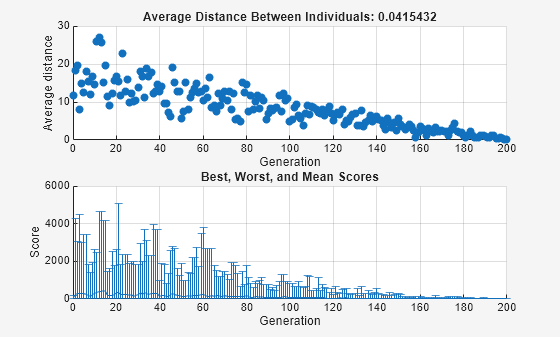
The upper plot displays the average distance between points in each generation. As the amount of mutation decreases, so does the average distance between individuals, which is approximately 0 at the final generation. The lower plot displays a vertical line at each generation, showing the range from the smallest to the largest fitness value, as well as mean fitness value. As the amount of mutation decreases, so does the range. These plots show that reducing the amount of mutation decreases the diversity of subsequent generations.

For comparison, the following figure shows the same plots when you set Shrink to 0.5.

options = optimoptions('ga',options,...
    'MutationFcn',{@mutationgaussian,1,.5});
[x,fval] = ga(@rastriginsfcn,2,[],[],[],[],[],[],[],options);

Optimization terminated: maximum number of generations exceeded.

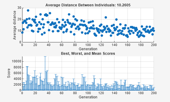
This time, the average amount of mutation decreases by a factor of 1/2 by the final generation. As a result, the average distance between individuals decreases less than before.

Setting the Crossover Fraction

The CrossoverFraction option specifies the fraction of each population, other than elite children, that are made up of crossover children. A crossover fraction of 1 means that all children other than elite individuals are crossover children, while a crossover fraction of 0 means that all children are mutation children. The following example show that neither of these extremes is an effective strategy for optimizing a function.

The example uses the fitness function whose value at a point is the sum of the absolute values of the coordinates at the points. That is,

$f (x_{1}, x_{2}, . . ., x_{n}) = | x_{1} | + | x_{2} | + \dots + | x_{n} | .$

You can define this function as an anonymous function by setting the fitness function to

fun = @(x) sum(abs(x));

Run the example with the default value of 0.8 as the CrossoverFraction option.

nvar = 10;
options = optimoptions('ga',...
    'InitialPopulationRange',[-1;1],...
    'PlotFcn',{@gaplotbestf,@gaplotdistance});
rng(14,'twister') % For reproducibility
[x,fval] = ga(fun,nvar,[],[],[],[],[],[],[],options)

Optimization terminated: average change in the fitness value less than options.FunctionTolerance.

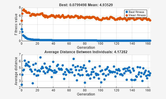
x = 1×10

   -0.0020   -0.0134   -0.0067   -0.0028   -0.0241   -0.0118    0.0021    0.0113   -0.0021   -0.0036

fval = 0.0799

Crossover Without Mutation

To see how the genetic algorithm performs when there is no mutation, set the CrossoverFraction option to 1.0 and rerun the solver.

options.CrossoverFraction = 1;
[x,fval] = ga(fun,nvar,[],[],[],[],[],[],[],options)

Optimization terminated: average change in the fitness value less than options.FunctionTolerance.

x = 1×10

   -0.0275   -0.0043    0.0372   -0.0118   -0.0377   -0.0444   -0.0258   -0.0520    0.0174    0.0533

fval = 0.3114

In this case, the algorithm selects genes from the individuals in the initial population and recombines them. The algorithm cannot create any new genes because there is no mutation. The algorithm generates the best individual that it can using these genes at generation number 8, where the best fitness plot becomes level. After this, it creates new copies of the best individual, which are then are selected for the next generation. By generation number 17, all individuals in the population are the same, namely, the best individual. When this occurs, the average distance between individuals is 0. Since the algorithm cannot improve the best fitness value after generation 8, it stalls after 50 more generations, because Stall generations is set to 50.

Mutation Without Crossover

To see how the genetic algorithm performs when there is no crossover, set the CrossoverFraction option to 0.

options.CrossoverFraction = 0;
[x,fval] = ga(fun,nvar,[],[],[],[],[],[],[],options)

Optimization terminated: average change in the fitness value less than options.FunctionTolerance.

x = 1×10

    0.4014    0.0538    0.7824    0.1930    0.0513   -0.4801    0.9988   -0.0059    0.0875    0.0302

fval = 3.0843

In this case, the random changes that the algorithm applies never improve the fitness value of the best individual at the first generation. While it improves the individual genes of other individuals, as you can see in the upper plot by the decrease in the mean value of the fitness function, these improved genes are never combined with the genes of the best individual because there is no crossover. As a result, the best fitness plot is level and the algorithm stalls at generation number 50.

Comparing Results for Varying Crossover Fractions

The example deterministicstudy.m, which is included when you run this example, compares the results of applying the genetic algorithm to Rastrigin's function with the CrossoverFraction option set to 0, 0.2, 0.4, 0.6, 0.8, and 1. The example runs for 10 generations. At each generation, the example plots the means and standard deviations of the best fitness values in all the preceding generations, for each value of the CrossoverFraction option.

Run the example.

deterministicstudy

Optimization terminated: average change in the fitness value less than options.FunctionTolerance.
Optimization terminated: average change in the fitness value less than options.FunctionTolerance.
Optimization terminated: average change in the fitness value less than options.FunctionTolerance.
Optimization terminated: average change in the fitness value less than options.FunctionTolerance.
Optimization terminated: average change in the fitness value less than options.FunctionTolerance.
Optimization terminated: average change in the fitness value less than options.FunctionTolerance.
Optimization terminated: average change in the fitness value less than options.FunctionTolerance.
Optimization terminated: average change in the fitness value less than options.FunctionTolerance.
Optimization terminated: average change in the fitness value less than options.FunctionTolerance.
Optimization terminated: average change in the fitness value less than options.FunctionTolerance.
Optimization terminated: average change in the fitness value less than options.FunctionTolerance.
Optimization terminated: average change in the fitness value less than options.FunctionTolerance.
Optimization terminated: average change in the fitness value less than options.FunctionTolerance.
Optimization terminated: average change in the fitness value less than options.FunctionTolerance.
Optimization terminated: average change in the fitness value less than options.FunctionTolerance.
Optimization terminated: average change in the fitness value less than options.FunctionTolerance.
Optimization terminated: average change in the fitness value less than options.FunctionTolerance.
Optimization terminated: average change in the fitness value less than options.FunctionTolerance.
Optimization terminated: average change in the fitness value less than options.FunctionTolerance.
Optimization terminated: average change in the fitness value less than options.FunctionTolerance.
Optimization terminated: average change in the fitness value less than options.FunctionTolerance.
Optimization terminated: average change in the fitness value less than options.FunctionTolerance.
Optimization terminated: average change in the fitness value less than options.FunctionTolerance.
Optimization terminated: average change in the fitness value less than options.FunctionTolerance.
Optimization terminated: average change in the fitness value less than options.FunctionTolerance.
Optimization terminated: average change in the fitness value less than options.FunctionTolerance.
Optimization terminated: average change in the fitness value less than options.FunctionTolerance.
Optimization terminated: average change in the fitness value less than options.FunctionTolerance.
Optimization terminated: average change in the fitness value less than options.FunctionTolerance.
Optimization terminated: average change in the fitness value less than options.FunctionTolerance.
Optimization terminated: average change in the fitness value less than options.FunctionTolerance.
Optimization terminated: average change in the fitness value less than options.FunctionTolerance.
Optimization terminated: average change in the fitness value less than options.FunctionTolerance.
Optimization terminated: average change in the fitness value less than options.FunctionTolerance.
Optimization terminated: average change in the fitness value less than options.FunctionTolerance.
Optimization terminated: average change in the fitness value less than options.FunctionTolerance.
Optimization terminated: average change in the fitness value less than options.FunctionTolerance.
Optimization terminated: average change in the fitness value less than options.FunctionTolerance.
Optimization terminated: average change in the fitness value less than options.FunctionTolerance.
Optimization terminated: average change in the fitness value less than options.FunctionTolerance.
Optimization terminated: average change in the fitness value less than options.FunctionTolerance.
Optimization terminated: average change in the fitness value less than options.FunctionTolerance.
Optimization terminated: average change in the fitness value less than options.FunctionTolerance.
Optimization terminated: average change in the fitness value less than options.FunctionTolerance.
Optimization terminated: average change in the fitness value less than options.FunctionTolerance.
Optimization terminated: average change in the fitness value less than options.FunctionTolerance.
Optimization terminated: average change in the fitness value less than options.FunctionTolerance.
Optimization terminated: average change in the fitness value less than options.FunctionTolerance.
Optimization terminated: average change in the fitness value less than options.FunctionTolerance.
Optimization terminated: average change in the fitness value less than options.FunctionTolerance.
Optimization terminated: average change in the fitness value less than options.FunctionTolerance.
Optimization terminated: average change in the fitness value less than options.FunctionTolerance.
Optimization terminated: average change in the fitness value less than options.FunctionTolerance.
Optimization terminated: average change in the fitness value less than options.FunctionTolerance.
Optimization terminated: average change in the fitness value less than options.FunctionTolerance.
Optimization terminated: average change in the fitness value less than options.FunctionTolerance.
Optimization terminated: average change in the fitness value less than options.FunctionTolerance.
Optimization terminated: average change in the fitness value less than options.FunctionTolerance.
Optimization terminated: average change in the fitness value less than options.FunctionTolerance.
Optimization terminated: average change in the fitness value less than options.FunctionTolerance.

Figure Genetic Algorithm contains 2 axes objects. Axes object 1 with title After 10 iterations, xlabel CrossoverFraction, ylabel Iteration contains an object of type image. Axes object 2 with xlabel CrossoverFraction, ylabel Score Mean and Std contains an object of type errorbar.

The lower plot shows the means and standard deviations of the best fitness values over 10 generations, for each of the values of the crossover fraction. The upper plot shows a color-coded display of the best fitness values in each generation.

For this fitness function, setting Crossover fraction to 0.8 yields the best result. However, for another fitness function, a different setting for Crossover fraction might yield the best result.