Environment
Live Editor Controls: Create dynamic controls in live scripts by linking variables to drop-down items and slider values
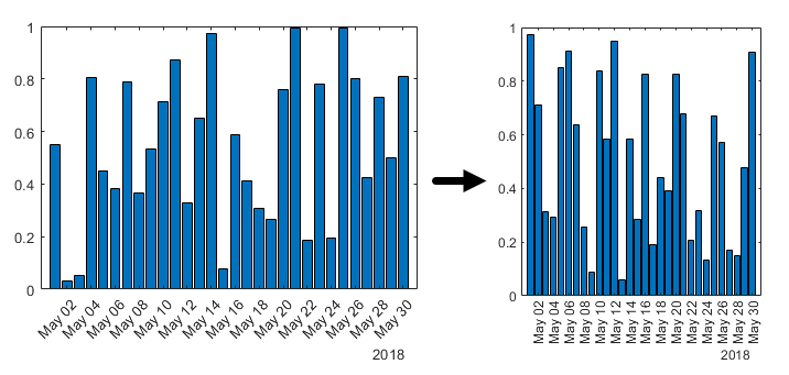
When adding a drop-down list to a live script, you can populate the items in it using values stored in a variable. When adding a slider, you can specify the minimum, maximum, and step values using variables.
For example, create a live script and define the variable lastnames
that contains a list of last
names.
lastnames = ["Houston","Vega","Obrien","Potter","Rivera","Hanson","Fowler","Tran","Briggs"];
Run the live script to create lastnames and add it to the
workspace. Then, go to the Live Editor tab, and in the
Code section, select Control > Drop Down. In the Items section of the control configuration
menu, select lastnames as the Variable.

Close the configuration menu to return to the live script. The drop-down list now
contains the last names defined in lastnames.
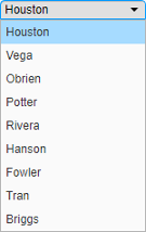
If you add, remove, or edit the values in lastnames, the items in
the drop-down list update accordingly.
For more information, see Add Interactive Controls to a Live Script.
Live Editor Fonts: Change the name, style, size, and color of fonts programmatically using settings
You can change the name, style, size, and color of titles, headings, text, and code in the Live Editor using settings.
For example, this code changes the color and style of titles in the Live Editor:
s = settings;
s.matlab.fonts.editor.title.Style.PersonalValue = {'bold'};
s.matlab.fonts.editor.title.Color.PersonalValue = [0 0 255 1];
This code increases the size and changes the font of normal text in the Live Editor:
s = settings;
s.matlab.fonts.editor.normal.Size.PersonalValue = 20;
s.matlab.fonts.editor.normal.Name.PersonalValue = 'Calibri';
The Live Editor updates all open live scripts and live functions to show the selected fonts. When you create new live scripts or functions, they use the new fonts as well.

For more information, see matlab.fonts.
Live Editor Display: Specify where to display output by default
You can change the default location for output in a new live script. Depending on this
preference, new live scripts that you create display their output inline or on the
right. To change the default, go to the Home tab, and in the
Environment section, select ![]() Preferences. Select MATLAB > Editor / Debugger > Display, and then select an option for the Live Editor default
view:
Preferences. Select MATLAB > Editor / Debugger > Display, and then select an option for the Live Editor default
view:
Output on right — Output displays to the right of the code. Each output displays next to the line that creates it. This option is ideal when writing code.
Output inline — Output displays inline with the code. Each output displays underneath the line that creates it. This option is ideal for sharing.
Live Editor Functions: Run live functions interactively using the Run button in MATLAB Online
In MATLAB®
Online™, you can now run live functions interactively using the
![]() Run button.
Run button.
To run live functions that require input argument values or any other additional
setup, configure the ![]() Run button by clicking Run
Run button by clicking Run![]() and adding one or more commands. For more information
about configuring the
and adding one or more commands. For more information
about configuring the ![]() Run button, see Configure the Run Button for Functions.
Run button, see Configure the Run Button for Functions.
Live Editor Bookmarks: Navigate quickly between lines
To navigate quickly between lines, set bookmarks in your live scripts or live functions. Bookmarks are particularly useful in long files when you frequently need to move between sections.
To set a bookmark, put the cursor on the line that you want to set it on. Then, go to
the Live Editor tab and, in the Navigate
section, click ![]() Bookmark. A bookmark icon
Bookmark. A bookmark icon ![]() appears to the left of the line. To clear a bookmark,
with the cursor on the line with the bookmark, click Bookmark
appears to the left of the line. To clear a bookmark,
with the cursor on the line with the bookmark, click Bookmark
![]() and select Set/Clear. You
also can clear the bookmark by clicking the bookmark icon
and select Set/Clear. You
also can clear the bookmark by clicking the bookmark icon ![]() to the left of the line.
to the left of the line.
To navigate to a bookmark, go to the Live Editor tab, and in the
Navigate section, click Bookmark
![]() . Then, select Previous or
Next.
. Then, select Previous or
Next.
For more information about navigating within files, see Go To Location in File.
Live Editor Animation Playback Controls: Interactive interface to control animations
Playback controls now appear within the figure window after an animation is done
playing. These playback controls provide the ability to replay the animation and explore
individual frames without having to re-run the entire live script. Animation playback
controls are not supported for animations generated by the movie
function.
Live Editor Performance: Improved performance when saving large live scripts or functions
When saving large live scripts or functions, you can continue using the Live Editor sooner in R2021a than in R2020b. While you continue to use the Live Editor, MATLAB saves the file in the background. When MATLAB finishes saving the file, the asterisk (*) next to the file name disappears, indicating that the file is saved.
For example, on a Windows® 10, Intel® Xeon® E5-1650 CPU @ 3.60 GHz test system, if you save a live script containing 35,000 lines of code and then click the title bar of another document open in the Live Editor, MATLAB immediately switches to the other open document. In R2020b, there is a noticeable delay before MATLAB switches to the other open document.
Help Browser: View web documentation by default
Starting in R2021a, when you run MATLAB with an internet connection, the Help browser displays the web documentation by default. When you run MATLAB on a system without an internet connection, or if your internet connection becomes unavailable, the Help browser displays the installed documentation instead.
To change the default documentation location, on the Home tab, in
the Environment section, click ![]() Preferences. Select MATLAB > Help and change the Documentation Location. For more
information, see Help Preferences.
Preferences. Select MATLAB > Help and change the Documentation Location. For more
information, see Help Preferences.
Documentation: View MATLAB documentation in French, Italian, and German
A subset of MATLAB documentation in French, Italian, and German is available on the web to licensed MATLAB users. Only a subset of the full documentation is available. For more information, see Translated Documentation.
MATLAB Drive: Get the location of your MATLAB Drive root folder programmatically
You can get the location of your MATLAB
Drive™ root folder programmatically, using the matlabdrive
command, from your desktop or in other MATLAB environments such as MATLAB
Online. For example, if you have MATLAB
Drive Connector installed on your desktop system, MATLAB returns the location of your MATLAB
Drive:
md = matlabdrive
md =
    'C:\Users\username\MATLAB Drive'
MATLAB Drive: Pause and resume syncing in MATLAB Drive Connector
You can temporarily stop the syncing of your MATLAB Drive files, for example, if you are on a metered or slow internet, by pausing and then resuming syncing.
For more information, see Use MATLAB Connector to Manage Your Files.
MATLAB Drive: MATLAB Drive Connector now available in Chinese and Korean
MATLAB Drive Connector now available in Chinese and Korean.
MATLAB Drive: Change the folder permissions for an invited member of a shared folder in MATLAB Drive Online (May 2021)
After inviting someone to access a shared folder, you can change the folder permissions for that person. For example, if you invite someone to share a folder as a read-only folder, you can change the permissions for that person to allow them to edit the contents of the folder.
For more information, see Share Files Using MATLAB Drive.
MATLAB Drive: Share folder by invitation to others who already have access to the folder through a view-only link (May 2021)
You can now invite others to access a shared folder even if they already have access to the folder through a view-only link. Inviting someone to access a shared folder allows you to give them edit permissions to the folder.
Functionality being removed or changed
PNG images in documentation are compressed
Behavior change
Starting in R2021a, all PNG images included in the documentation are compressed, reducing their stored size on disk. The compressed images should be visually identical to the original images.
Language and Programming
Name=Value Syntax: Use name=value syntax for passing name-value arguments
MATLAB supports a new syntax for passing name-value arguments. In the new syntax, the name and value arguments are connected by an equal sign, and the name is not enclosed in quotes.
Name=value syntax:
plot(x,y,LineWidth=2)
Comma-separated syntax:
plot(x,y,"LineWidth",2)
MATLAB continues to support the comma-separated name,value
syntax. Existing functions and methods support both syntaxes, and the process for
writing functions and methods with name-value arguments is unchanged.
Use the new syntax to help identify name-value arguments for functions and to
distinguish names from values in lists of name-value arguments. There are some
limitations on where and how the name=value syntax can be
used:
The recommended practice is to use only one syntax in any given function call. However, if you do mix
name=valueandname,valuesyntaxes in a single call, allname=valuearguments must appear after thename,valuearguments. For example,plot(x,y,"Color","red",LineWidth=2)is a valid combination, butplot(x,y,Color="red","LineWidth",2)errors.Similarly,
name=valuearguments must appear after all positional arguments. CallingmyFunction(name=value,posArgument)errors.The
name=valuesyntax can only be used directly in function calls. They cannot be wrapped in a cell array or additional parentheses. CallingmyFunction(a,(name=value))errors.
Retrieving Display Format: format function can get and set
display format
The format function can now output the current Command Window
display format. Calling format with an output variable returns a
DisplayFormatOptions object that describes the current numeric and
line spacing
formats:
fmt = format
fmt =
   DisplayFormatOptions with properties:

         NumericFormat: "shortE"
           LineSpacing: "loose"
You can also use a DisplayFormatOptions object as an input to
format to change the display format.
Capturing disp Output: Use the
formattedDisplayText function to store
disp output as a string
formattedDisplayText captures the output of
disp(obj) as a string. The function also enables you to control
the formatting of the captured string, including numeric format and line spacing. For
example, A is a vector containing three logical values.
formattedDisplayText displays the vector elements as the words
“true” or
“false”:
out = formattedDisplayText(A,"UseTrueFalseForLogical",true) out =
' true false true
'Virtual File Storage: mkdir and rmdir will now
be able to create and remove files from VFS directories
Starting in R2021a, rmdir and mkdir are able to
create folders in remote locations.
Function Argument Validation: Debugger and profiler is now supported
The MATLAB debugger will now be usable inside of the arguments
blocks of functions. While debugging an arguments block the workspace
is read only. The MATLAB profiler will now record lines inside of arguments blocks.
Class Diagram Viewer: Create graphical class diagrams to explore class details and share designs
Use the Class Diagram Viewer tool to create graphical class diagrams, including details such as:
Inheritance relationships, including abstract classes, mixins, and multiple inheritances
Lists of properties, methods, and events
Class member access levels
You can use the diagrams to explore complex class designs. You can also use the diagrams to share proposed designs with team members, either as static images or editable diagrams.
Use the associated matlab.diagram.ClassViewer class for command line
access to diagrams.
Enumeration Comparisons: Use isequal to compare enumeration members
with text data types
Enumeration classes now have a default implementation of the isequal
method. You can use isequal to compare enumeration members with
character vectors, strings, and cell arrays of character vectors or strings. For more
information, see isequal Method.
eval function: Context checking to resolve identifiers
MATLAB now resolves identifiers like variable names in an eval
statement using additional context. For instance, MATLAB recognizes when a call to eval uses a variable declared
in a function.
With the additional context, MATLAB resolves ambiguities differently than in previous releases. Some code now produces errors or warnings.
Code that warns starting in R2021a will error in a future release.
| Example | Previous Result | R2021 Result | Notes |
|---|---|---|---|
function myfun(pi) eval('pi') end >> myfun |
ans = 3.1416 | Errors | MATLAB resolves |
function myfun disp(pi) eval('pi = 1'); end >> myfun |
3.1416 pi = 1 | Same output but warns on assignment. | MATLAB resolves In a future release,
function myfun disp(pi) pi = 1; end |
% assignLocal.m script: local = 1; % myfun.m file with local function: function myfun local() assignLocal eval("local") end function local disp("local fx") end % function call: >> myfun |
local fx local = 1 | Same output but warns on assignment. | In a future release, MATLAB will give precedence as described in Function Precedence Order. In this example, precedence goes to the local function. This new behavior is consistent with processing the following code: function myfun local() assignLocal local() end |
Functionality being removed or changed
format with no arguments is not recommended
Still runs
The format command, by itself, resets the output display
format to the default, which is the short, fixed-decimal format for floating-point
notation and loose line spacing for all output lines.
format
For clearer code, explicitly specify the default style.
format defaultDefining classes and packages: Using schema.m will not be
supported in a future release
Still runs
Support for classes and packages defined using schema.m files
will be removed in a future release. Replace existing schema-based classes with
classes defined using the classdef keyword.
compose does not accept an invalid hexadecimal value, octal
value, or trailing backslash
Errors
Previously, when the formatSpec input to compose contained an
invalid hexadecimal value, octal value, or trailing backslash it would issue a
warning and truncate the output at the point of the invalid value. Starting in
R2021a, MATLAB will issue an error instead. With this change, compose will error for
all invalid formatSpec inputs.
Using get and set to access or change
display format is not recommended
Still runs
Using get and set to programmatically
access or change the numeric display format and the display line spacing is not
recommended. Use settings instead. For example:
s = settings;
myformat = s.matlab.commandwindow.NumericFormat.ActiveValue
myformat =
    'short'
s.matlab.commandwindow.DisplayLineSpacing.TemporaryValue = 'compact';
myspacing = s.matlab.commandwindow.DisplayLineSpacing.ActiveValuemyspacing =
'compact'For more information, see matlab.commandwindow Settings.
Using feature('EightyColumns') to access and change Command
Window display width is not recommended
Still runs
Using the command feature('EightyColumns') or
feature('EightyColumns',
to programmatically determine or change whether the Command Window display width
limit is enabled is not recommended. Use settings instead. For example:value)
s = settings;
s.matlab.commandwindow.UseEightyColumnDisplayWidth.TemporaryValue = 1;
limitwidth = s.matlab.commandwindow.UseEightyColumnDisplayWidth.ActiveValue
limitwidth =
  logical
   0
For more information, see matlab.commandwindow Settings.
Data Analysis
Data Preprocessing Live Editor Tasks: Operate on multiple table variables and specify output format for table input
When you are working with data in a table or timetable, these Live Editor tasks now allow you to operate on multiple table variables at the same time:
You can also choose which variable to display when visualizing the results.
In addition, tasks that modify variables provide new output options. You can return a table with all of the variables, or with only the variables that were modified. For tasks that return logical arrays, you can specify the size of the output. The size can match the size of the input table or a table containing only the variables that were used in the calculation.
Clean Outlier Data Live Editor Task: Visualize results with a histogram
The Clean Outlier Data Live Editor task now offers histogram plots for most detection methods. The histogram can summarize the input data, the outliers, the cleaned data with the outliers filled, and the outlier detection thresholds and center value.
fillmissing Function: Specify custom fill method
You can now specify a custom method for filling missing values when using the
fillmissing function. Specify the custom method as a function
handle.
normalize Function: Normalize multiple data sets with same
parameters
normalize can now return the centering and scaling parameter values used
to perform the normalization. You can reuse these parameters to normalize subsequent
data sets in the same manner. For example, you can normalize an array of data
A and then normalize a second array B with the
same
parameters:
[Anorm,C,S] = normalize(A);
Bnorm = normalize(B,'center',C,'scale',S);
The new outputs C and S contain the centering
and scaling parameter values, respectively. So that you can easily reuse them in a later
normalization step, you can also now specify the 'center' and
'scale' normalization methods at the same time. These are the
only two normalization methods that you can specify together.
To further support these changes, when method is
'center' or 'scale', the possible values of
methodtype now include arrays and tables. While these
methodtype values are intended to work with the new outputs
C and S, you also can compute your own
normalization parameters to specify.
groupcounts Function: Display percentages of group
counts
groupcounts now displays information about the percentage each group
count represents.
For table and timetable inputs,
groupcountsautomatically displays the percentages represented by each group count in the output table.For array inputs,
groupcountshas a new third output argument to return the percentages represented by each group count.
When groupcounts operates on data in a table or timetable,
the output contains an additional table variable for the percentages. The
percentages are in the range [0 100] and are included in the
table variable Percent.
Any code that references specific table variables is unaffected. However, you might need to update code that depends on the number of variables in the output table.
ts2timetable Function: Convert timeseries
objects to timetables
To convert timeseries objects to timetables, use the ts2timetable function.
table and timetable Functions: Specify
dimension names using the 'DimensionNames' name-value
argument
When you create tables and timetables, you can specify their dimension names by using
the 'DimensionNames' name-value argument with these functions:
In previous releases, you could change the dimension names only by creating a table or
timetable and then changing its DimensionNames property.
Functionality being removed or changed
Table dimension names cannot match reserved names
Behavior change
MATLAB raises an error if you assign a dimension name that matches one of
these reserved names: 'Properties',
'RowNames', 'VariableNames', or
':'. In previous releases, MATLAB raised a warning and modified the dimension names so that they were
different from the reserved names.
For example, if you create a table and then assign 'Properties'
as a dimension name, the result is an error.
T = array2table(magic(3));
T.Properties.DimensionNames = {'Rows','Properties'}
'SamplingRate' will be removed
Warns
The 'SamplingRate' name-value argument will be removed in a
future release. Use 'SampleRate' instead. The corresponding
timetable property is also named SampleRate.
For backward compatibility, you still can specify
'SamplingRate' as the name of the name-value argument.
However, the value is assigned to the SampleRate
property.
This change in behavior affects the timetable functions shown in the list:
Data Import and Export
XML Files: Read, write, and import XML files using readtable,
readtimetable, and other functions
The readtable, writetable,
readtimetable, writetimetable, and
detectImportOptions functions now support reading and writing XML
files. This list outlines the added capabilities of each function.
readtableandreadtimetable— Read XML data into MATLAB as a table or timetable. You can specify optional name-value arguments to control howreadtableandreadtimetabletreat XML data. For example, specify‘ImportAttributes’,falseto ignore attribute nodes.writetableandwritetimetable— Write a table or timetable in MATLAB to an XML file. Specify optional name-value arguments to control howwritetableandwritetimetabletreat XML data. For example, specify‘AttributeSuffix','_att'to specify that all table or timetable variables with the suffix'_att'should be written as attributes in the output XML file.detectImportOptions— ThedetectImportOptionsfunction now returns anXMLImportOptionsobject when you call it on an XML file. Its behavior when you call it on other file types has not changed. Use theXMLImportOptionsobject withreadtableto customize import options. For instance:Import only a subset of data using the
SelectedVariableNamesproperty.Specify the names and data types of the variables in the input file using the
VariableNamesand theVariableTypesproperties.Manage the import of specific nodes in the XML file using name-value arguments such as
'TableSelector','RowSelector', or'VariableSelectors'.
For more information, see XMLImportOptions.
MATLAB API for Advanced XML Processing: Create, read, write, transform, and query XML
Use the MATLAB API for XML Processing (MAXP) to develop advanced applications that create, read, write, transform, and query XML documents. MAXP consists of these packages:
matlab.io.xml.dom— Classes for creating, reading, and writing XML files and strings following the W3C DOM standard.matlab.io.xml.transform— Classes for transforming XML documents from one type to another following the XSLT 1.0 standard.matlab.io.xml.xpath— Classes for querying XML documents using XPath 1.0 expressions.
XML Files: Register XML namespace prefixes for evaluating XPath expressions using
readtable,readstruct, and other
functions
Use the RegisteredNamespaces name-value argument to specify
namespace prefixes that readtable, readtimetable,readstruct, XMLImportOptions, and detectImportOptions use when evaluating XPath expressions in an XML
file. RegisteredNamespaces can be used when you also evaluate an
XPath expression specified by a selector name-value argument, such as
StructSelector for readstruct, or
VariableSelectors for readtable and
readtimetable.
The readstruct function automatically detects namespace prefixes to
register for use in XPath evaluation, but you can also register new namespace prefixes
using the RegisteredNamespaces name-value argument. You might
register a new namespace prefix when an XML node has a namespace URL, but no declared
namespace prefix in the XML file. In that case, you can specify
RegisteredNamespaces as a string array containing a namespace
prefix and the associated URL.
For example, evaluate an XPath expression on an XML file named
example.xml which does not contain a namespace prefix
declaration. Specify 'RegisteredNamespaces' as [“myprefix”,
“https://www.mathworks.com”] to assign the prefix
myprefix to the URL
https://www.mathworks.com.
data = readstruct("example.xml", "StructSelector", "/myprefix:Data",...
 "RegisteredNamespaces", [“myprefix”, “https://www.mathworks.com”])
In the resulting structure, the namespace prefix and URL will appear as attributes
belonging to the element specified in the StructSelector name-value
argument.
Low-level file I/O functions and remote data: Perform read and write operations on remotely stored files
You can now use low-level file I/O functions, such as fopen, fread, and fwrite, to work with files stored in remote locations. Some supported
remote locations include Amazon S3™ and Windows Azure® Blob Storage.
When reading from or writing to a remote location, you must specify the full path using a uniform resource locator (URL). For example, open a binary file from the Amazon S3 cloud.
fid = fopen(“s3://bucketname/path_to_file/example.bin”);
For more information on setting up MATLAB to access your online storage service, see Work with Remote Data.
save and load functions and remote data: Save,
load, and append data to remotely stored v7.3 MAT-files
You can now access v7.3 MAT-files stored in remote locations, such as Amazon S3 and Windows Azure Blob Storage, using the save and load functions.
When saving, loading, or appending data to a remote location, you must specify the full path using a uniform resource locator (URL). For example, load a MAT-file from the Amazon S3 cloud.
load(“s3:://bucketname/path_to_file/example.mat”);
For more information on setting up MATLAB to access your online storage service, see Work with Remote Data.
Reading Online Data: Read files over HTTP and HTTPS using
readtable, audioread, and other reading
functions
Read files from an internet URL by specifying filename as a string
that contains the protocol type 'http://' or
'https://'. This lets you read data from their primary online
sources.
This functionality is supported by these functions: audioread,
audioinfo, parquetread,
parquetinfo, readtable,
readtimetable, readvars,
readstruct, readmatrix,
readcell, readlines, and
detectImportOptions.
Parquet Data Format: Use categorical data in parquet data format
Read, write, and analyze parquet data that contain the categorical
data type.
This functionality is supported by these functions: parquetread,
parquetwrite, parquetinfo, and
parquetDatastore.
Datastores: Read all data from a datastore using parallel processing
You can use parallel processing when reading all data from a datastore (requires Parallel Computing Toolbox™). Parallel processing results in improved performance when reading data, especially with remote data.
Data Compression Functions: Improved functionality in
zip/unzip and
tar/untar
On Windows, macOS, and Linux® systems:
zipcan compress an individual file of any size.zipcan compress any number of files in a single function call.tarcan compress a group of files of any cumulative size.
Additionally, on Windows systems, unzip and untar replace
invalid characters with underscores if they occur in entry path names of the original
file.
imfinfo function: Get information about all Adobe Digital Negative (DNG) file tags
The imfinfo function returns information on all DNG file tags as individual
named fields in the output structure. For a complete list of DNG file tags, see Chapter
4 of the Adobe® Digital Negative (DNG) Specification.
jsonencode: Add indentation to JSON text
Use the jsonencode
'PrettyPrint' option to display JSON text with an indentation of two
spaces.
s.Width = 800;
s.Height = 600;
s.Title = 'View from the 15th Floor';
s.Animated = false;
s.IDs = [116, 943, 234, 38793];
jsonencode(s,'PrettyPrint',true)
ans =
    '{
       "Width": 800,
       "Height": 600,
       "Title": "View from the 15th Floor",
       "Animated": false,
       "IDs": [
         116,
         943,
         234,
         38793
       ]
     }'
Functionality being removed or changed
The H5I.get_name function only accepts named HDF5 datatypes as
input arguments.
Behavior change
Starting in R2020a, the H5I.get_name function only accepts
committed (previously called named) HDF5 datatypes as input
arguments, and will error if you pass other datatypes as input. In releases R2019b
and earlier, H5I.get_name does not error if you pass other
datatypes as input.
To verify that the input is a committed HDF5 datatype, call the
H5T.committed function on it. The
H5T.committed function returns a value of
1 if the input is a committed HDF5 datatype, and a value of
0 if it is not.
imfinfo now returns Adobe DNG tags belonging to versions 1.2 through 1.5 in individual named
fields in the output structure
Behavior change
When you call the imfinfo function on an Adobe DNG file, it now returns tags belonging to versions 1.2 through 1.5 as
individual named fields in the output structure. Previously, tags belonging to these
versions were stored in the 'UnknownTags' field of the output
structure. For a complete list of DNG file tags, see Chapter 4 of the Adobe Digital Negative (DNG) Specification.
imread reads the first frame in a GIF file by default
Behavior change
Starting in R2021a, when you read a GIF file without specifying additional
arguments, the imread function reads the first frame by default.
Previously, imread read all the frames in the file by
default.
To read all the frames in the order that they appear in the GIF file, specify the
value of the 'Frames' name-value argument as
'all'.
serial function will be removed
Still runs
serial and its object properties will be removed. Previously,
serial and its object properties were not recommended. Use
serialport and its properties instead.
This example shows how to connect to a serial port device using the recommended functionality.
| Functionality | Use This Instead |
|---|---|
s = serial("COM1");
s.BaudRate = 115200;
fopen(s) |
s = serialport("COM1",115200); |
See Transition Your Code to serialport Interface for more
information about using the recommended functionality.
Mathematics
Graph Algorithms: Compute all paths, all cycles, and cycle basis
graph and digraph objects have new functions to compute paths and cycles:
allpaths— Compute all paths between two nodes in agraphordigraphobject.allcycles— Compute all cycles in agraphordigraphobject.cyclebasis— Compute the fundamental cycle basis of agraphobject.hascycles— Determine whether agraphordigraphobject contains cycles.
griddedInterpolant Object: Use multivalued interpolation to
interpolate multiple data sets simultaneously
griddedInterpolant can now interpolate multiple data sets on the same grid
at the same query points. For example, if you specify a 2-D grid, a 3-D array of values
at the grid points, and a 2-D collection of query points, then
griddedInterpolant returns the interpolated values at the query
points for each 2-D page in the 3-D array of values.
Previously, this functionality was available in interp1 for 1-D
interpolation, but this improvement to griddedInterpolant adds support
for N-D multivalued interpolation.
eig Function: Improved algorithm for skew-Hermitian
matrices
eig now has an improved algorithm for input matrices that are
skew-Hermitian. With the function call [V,D] = eig(A), where
A is skew-Hermitian, eig now guarantees that
the matrix of eigenvectors V is unitary and the diagonal matrix of
eigenvalues D is purely imaginary.
cdf2rdf Function: Improved algorithm for all inputs
cdf2rdf has an improved algorithm for all input matrices that reduces
floating-point round-off errors in the calculation.
Functionality being removed or changed
Line Continuation: Ellipsis following operator treated as a space
Behavior change
Previously, if an ellipsis followed an operator inside of a matrix or cell array, it caused the operator to be treated as unary. Ellipses will now be treated as a space in all cases.
| Old Behavior | New Behavior |
|---|---|
x = [1 -...
2]
x =
1 -2Previously,
this code was equivalent to the expression, | x = [1 -...
2]x =
-1Now,
the ellipsis will be treated as a space so this code is
equivalent to the expression, |
Graphics
Create Plot Live Editor Task: Create plots interactively and generate code
The Create Plot Live Editor Task makes generating and exploring visualizations for data simple and interactive. With this task you can select the data you wish to visualize and choose the plot type that best represents that data. Alternatively, you can explore the visualizations available in MATLAB to find the desired plot type and add your data. This task creates labels for the visualization based on the data and can be used to add or adjust the optional parameters of the visualization.
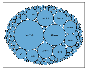
bubblecloud Function: Visualize part-to-whole
relationships
Use the bubblecloud function to illustrate the relationship between elements in
your data set and the set as a whole. For example, you can visualize data collected from
different cities, and represent each city as a bubble whose size is proportional to the
value for that city.
tiledlayout Function: Control the tile indexing scheme
Control whether the tile indices increase across the rows or down the columns of a
layout by setting the TileIndexing property of a TiledChartLayout object.
Select one of the following options:
'rowmajor'— Increment the tile indices across the first row before moving to the next row. This is the default behavior.'columnmajor'— Increment the indices down the first column before moving to the next column. This indexing scheme is the same as linear indexing for arrays.
The nexttile function populates tiles according to
the indexing scheme. If you change the tile indexing of a populated layout, the tile
positions change to match the new scheme.
PolarAxes Objects: Use the CurrentPoint
property or call ginput to get the cursor location within polar
axes
Query the CurrentPoint property of a PolarAxes object to get
the location of the last click within the axes. The ginput function also supports querying coordinates of polar axes.
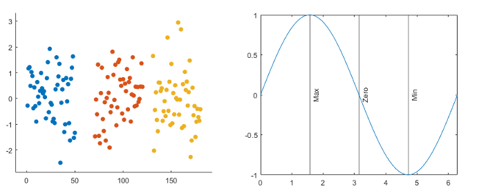
Scatter Plots and Constant Lines: Create multiple scatter plots or constant lines at once
The
scatter,polarscatter, andswarmchartfunctions now accept the same combinations of matrices and vectors as theplotfunction does. As a result, you can visualize multiple data sets at once rather using theholdfunction between plotting commands.The
xlineandylinefunctions now accept vectors of values for creating multiple vertical or horizontal reference lines. You can also specify separate labels for each line using a string array or a cell array.
Axis Limits: Define LimitsChangedFcn callback that executes when
the limits of an axis change
Define the LimitsChangedFcn callback function on any type of ruler object such as a
numeric ruler. The callback function executes when the limits of the corresponding axis
change. For example, you can define the callback in an app to update another aspect of
the UI when the user pans within the axes.
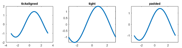
Axis Limits: Control axis limits
Control the axis limits for your plots by setting the XLimitMethod,
YLimitMethod, or ZLimitMethod on the axes.
Select one of the following property values:
'tickaligned'— Align the edges of the axes box with the tick marks that are closest to your data without excluding any data. This is the default option.'tight'— Fit the axes box tightly around the data by setting the axis limits equal to the range of the data.'padded'— Fit the axes box around the data with a thin margin of padding on each side. The width of the margin is approximately 7% of your data range.
exportgraphics and copygraphics Functions:
Specify RGB, CMYK, or grayscale output
Choose a color space when exporting or copying graphics. Specify the
Colorspace name-value argument when you call the exportgraphics or copygraphics functions. Select one of the following options:
'rgb'— Capture truecolor RGB content. This is the default color space.'gray'— Convert the content to grayscale.'cmyk'(exportgraphicsonly) — Convert the content to cyan, magenta, yellow, and black (CMYK) before exporting the content as an EPS file.
colororder Function: Control colors in stacked plots
The colororder function now supports charts created with the stackedplot function.
Tick Labels: Automatically rotate tick labels
When you manually specify the ticks or the tick labels for a chart, the tick labels automatically rotate to give the best possible presentation given the size of the figure and the number of the tick labels.
patch and errorbar Functions: Expanded data
type support
The patch and errorbar functions now support more data types:
The
patchfunction accepts numeric, datetime, duration, and categorical values for the x-, y-, and z-coordinates.The
errorbarfunction accepts numeric, datetime, duration, and categorical values for the x- and y-coordinates. It also accepts numeric and duration values for the error bar lengths above, below, and on either side of the data points.
Geographic Plots: Access basemaps using additional proxy server authentication types
You can now access basemaps for geographic axes and charts using additional proxy server authentication types.
On Windows, you can use Basic, Digest, NTLM, Negotiate (SPNEGO), and Kerberos authentication.
On Linux and macOS, you can use Basic, Digest, and NTLM authentication.
Prior to R2021a, geographic axes and charts supported only types without authentication or with Basic authentication. For more information about specifying proxy server settings, see Use MATLAB Web Preferences For Proxy Server Settings.
Functionality being removed or changed
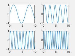
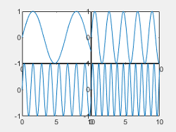
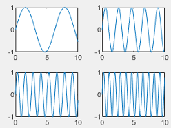
Tile spacing and padding options for tiled chart layouts have changed
Behavior change
When you create a tiled chart layout, some of the TileSpacing
and Padding properties provide a different result or have new
names.
The new TileSpacing options are 'loose',
'compact', 'tight', and
'none'. The new Padding options are
'loose', 'compact', and
'tight'. The following tables describe how the previous
options relate to the new options.
TileSpacing
Changes
Previous TileSpacing Option | R2021a TileSpacing Option | How to Update Your Code |
|---|---|---|
|
| Consider changing instances of
The
|
|
| No changes needed. |
| Not Applicable |
|
|
|
| The To preserve
the spacing between the plot boxes, change instances of
|


Padding Changes
Previous Padding Option | R2021a Padding Option | How to Update Your Code |
|---|---|---|
|
| Consider changing instances of
The
|
|
| No changes needed. |
|
| Consider changing instances of
The
|
Passing an empty label to the legend function omits the entry
from the legend
Behavior change
When you call the legend function and specify a label as an empty character vector, an
empty string, or an empty element in a cell array or string array, the corresponding
entry is omitted from the legend. In R2020b and earlier releases, the entry appears
in the legend without a label.
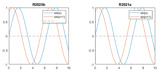
For example, this code plots two sine waves and a reference line at
y=0. Then it creates a legend with three labels, where the
last label is empty. In R2020b, the third line appears in the legend without a
label. In R2021a, the third line is omitted from the legend.
x = 0:0.2:10;
plot(x,sin(x),x,sin(x+1));
hold on
yline(0,'--')
legend('sin(x)','sin(x+1)','')
To keep an entry in the legend without a label, include a space character in the
label. For example, to update the preceding code, specify the last label as a
character vector containing a space ('
').
legend('sin(x)','sin(x+1)',' ')
Alternatively, if you do not want to display a space character, you can pass the
individual line objects to the legend function with an array of
labels. To get the individual line objects, call each plotting function with an
output
argument.
x = 0:0.2:10;
p = plot(x,sin(x),x,sin(x+1));
hold on
line0 = yline(0,'--');
legend([p(1) p(2) line0], {'sin(x)','sin(x+1)',''});
The XData, YData, and
ZData properties on Patch objects
created with the fill and fill3 functions
return values of the original data type
Behavior change
The XData, YData, and
ZData properties on a Patch object
created by the fill or fill3 functions return the coordinates using the original input data
type, rather than returning them as double values.
In previous releases, datetime, duration, and categorical coordinates are
converted to double values when they are stored in the
XData, YData, and
ZData properties.
For example, this code creates a filled polygon with datetime
x-coordinates. Then it calculates x2 using the
values stored in the XData property. In R2020b,
h.XData and x2 are
double arrays. In R2021a, h.XData and
x2 are datetime
arrays.
x = datetime('01-Jan-2018') + days([0 1 1 0]);
y = [0 0 1 1];
h = fill(x,y,'red');
x2 = h.XData + 1;
To preserve the double values in your code, get the
double values from the Vertices property
of the Patch object. The x-,
y-, and z-coordinates are stored as
double values in the first, second, and third columns of the
Vertices
array.
x2 = h.Vertices(:,1) + 1;
Alternatively, use the ruler2num function. Pass the coordinate values and the corresponding
axis ruler to the ruler2num
function.
ax = gca;
x2 = ruler2num(h.XData,ax.XAxis) + 1;
Graphics objects and UI components sized using 'points',
'inches', and 'centimeters' units will
increase in size on macOS platforms
Behavior change in future release
In a future release, graphics and UI objects that have Units or
FontUnits properties set to 'points',
'inches', or 'centimeters' will use a
conversion value of 1 pixel = 1/96th inch on macOS platforms. The current conversion value is 1 pixel = 1/72nd inch. As a
result, these objects and text elements will display 1.33 times larger than their
previous size. This change will provide a more readable default font size and will
ensure a consistent object size across Windows and macOS platforms.
The following objects use a unit value of 'pixels' by default
and will not be affected by this change:
UI components in App Designer or in apps created with the
uifigurefunctionUI components in apps created in GUIDE and migrated to App Designer using the GUIDE to App Designer Migration Tool for MATLAB
Axes objects created using the
uiaxesfunction
For the most control when sizing and laying out your graphics objects and UI
components, use a value of 'pixels' for Units
and FontUnits properties. To maintain object sizes in current and
future releases, make these updates in your code:
Objects with
UnitsorFontUnitsset to'points'— Update the value of the property from'points'to'pixels'.Objects with
UnitsorFontUnitsset to'inches'— Update the value of the property from'inches'to'pixels'and multiply allPositionvalues by 72.Objects with
UnitsorFontUnitsset to'centimeters'— Update the value of the property from'centimeters'to'pixels'and multiply allPositionvalues by 72/2.54.
For example, this code creates a push button in a figure window, with its position specified in inches:
uicontrol('Units','inches','Position',[0.6 0.1 1.75 0.5]);
In a future release, the push button created by this code will display 1.33 times larger on macOS platforms. To maintain the size and position of the push button in current and future releases, update the code to:
uicontrol('Units','pixels','Position',[50 10 126 36]);
Align Distribute Tool will be removed in a future release
Warns
The Align Distribute Tool will be removed in a future release.
To control the arrangement of multiple plots in a figure, create a tiled chart
layout using the tiledlayout function instead.
To align or distribute graphics objects within a figure, select Tools > Align or Tools > Distribute from the figure toolbar instead.
App Building
uihyperlink Function: Add and configure clickable links in apps
and on the App Designer canvas
To create a link, call the uihyperlink function or, in App Designer, drag a hyperlink UI component
from the Component Library onto the canvas.
Hyperlink UI components are supported only in App Designer apps and in figures created
with the uifigure function.
uitree Function: Add and configure check box trees in apps and on
the App Designer canvas
A check box tree is a styled with check boxes to the left of every item. You can now create check box trees in apps and on the App Designer canvas. Check box trees allow for easier selection of multiple tree nodes.
In apps created programmatically with the uifigure function, create a check box tree using the uitree function by specifying the style
'checkbox'.
In App Designer, create a check box tree by dragging it from the Component Library onto the canvas.
Interpreter Property: Style text and display equations in labels
with HTML and LaTeX markup
Use the Interpreter property on Label objects
(created with the uilabel function) to enable markup in the label text. To add HTML
markup, set the Interpreter property to 'html'. To
add LaTeX markup, set the Interpreter property to
'latex'.
For more information, see Label Properties.
WindowStyle Property: Create UI figures that remain in the
foreground
To keep a specific UI figure window in front of other windows, set the
WindowStyle property to 'alwaysontop'. Unlike
modal figures, UI figure windows with this property setting do not restrict keyboard and
mouse interactions.
The 'alwaysontop' property value is available only in figures
created using the uifigure function.
For more information, see UI Figure Properties.
scroll Function: Scroll to a location within a table UI component
programmatically
Use the scroll function to scroll within a table UI component programmatically.
Specify the scroll location as the top, bottom, left, or right side of the table, or as
a specific row, column, or table cell.
UI Component Accessibility: Select ListBox items,
Table cells, ColorPicker colors, and
DatePicker menus using the keyboard
You can now use keyboard shortcuts to change the focus and make selections in various
UI components. These shortcuts are supported for components in figures created using
the uifigure function.
| Component | Action | Keyboard Shortcut |
ListBox with Multiselect
property set to 'off' | Toggle list box selection. | Space |
ListBox with
Multiselect property set to
'on' | Select all items. | Ctrl+A |
| Move focus to previous item and toggle selection. | Shift+Up | |
| Move focus to next item and toggle selection. | Shift+Down | |
| Move focus to previous item without toggling selection. | Ctrl+Up | |
| Move focus to next item without toggling selection. | Ctrl+Down | |
| Toggle selection of item currently in focus. | Ctrl+Space | |
Table | Select table cell in top-left corner. | Ctrl+Home |
| Select table cell in bottom-right corner. | Ctrl+End | |
ColorPicker gradient selector | Move gradient selector. | Arrow keys |
ColorPicker hue slider | Move hue slider. | Up and Down |
DatePicker | Cycle between drop down menus, buttons, and calendar. | Tab |
App Designer: Use custom UI components in App Designer
You can now configure custom UI component classes to appear in the App Designer Component Library and to be used interactively in Design View.
To configure a custom UI component class for use in App Designer, follow these steps:
Define your own UI component class by creating a subclass of the
matlab.ui.componentcontainer.ComponentContainerbase class.Call the
appdesigner.customcomponent.configureMetadatafunction and specify the path to the component class.mfile.Use the resulting dialog box to configure the metadata associated with the component, including the component name, icon, author, and category.
This creates a resources folder with the App Designer
metadata. To view the component in the App Designer Component
Library, add the folder containing the component class file and the
generated resources folder to the MATLAB path.
To share your custom UI component for others to use in App Designer, share both the
component class file and the resources folder.
For more information, see Configure Custom UI Components for App Designer.
App Designer: Zoom and pan in the canvas, and zoom in the Code View editor
To zoom in or out in the App Designer canvas and in the Code View editor, hold Ctrl and move the scroll wheel, or press Ctrl+Plus and Ctrl+Minus. To return to the default scale, press Ctrl+Alt+0. Zooming does not affect the Component Library, Component Browser, or Code Browser.
To pan in the App Designer canvas, use one of the following:
Click and drag with the middle mouse button.
Hold Space while clicking and dragging with the left mouse button.
In previous releases, the Ctrl+Plus and Ctrl+Minus keyboard shortcuts zoomed the entire App Designer desktop.
App Designer: Control color and tab settings in Code View using MATLAB preferences
Color and tab preferences applied to the MATLAB Editor are now also applied to the App Designer Editor.
Additionally, you can now change the background color of the App Designer read-only code. Access this setting in the App Designer tab of MATLAB preferences.
For more information, see Personalize Code View Appearance.
App Designer: Customize split-screen layouts in the App Designer editor
To view your document in horizontal or vertical split-screen mode in the App Designer Code View editor, select a layout in the App Designer toolstrip.
App Testing Framework: Perform gestures on panels and tables
The app testing framework supports gestures on more UI components:
Perform
press,hover, andchooseContextMenugestures on panels.Perform
choose,type, andchooseContextMenugestures on table UI components.
App Testing Framework: Close alert dialog box in front of figure window
You can now use the dismissAlertDialog method as part of a test case to programmatically close
an alert dialog box in front of a figure window. For example, create a modal alert
dialog box and close it by calling the
method.
fig = uifigure;
uialert(fig,'File not found','Invalid File')

tc = matlab.uitest.TestCase.forInteractiveUse;
tc.dismissAlertDialog(fig)
Web Apps and Standalone Applications: Datatips supported in graphics
Graphics created in web apps and standalone applications support datatips. Use datatips in these applications just as you would in MATLAB figures.
Functionality Being Removed or Changed
GUIDE will be removed in a future release
Warns
The GUIDE environment and the guide function will be removed in a future release.
After GUIDE is removed, existing GUIDE apps will continue to run in MATLAB but will not be editable using the drag-and-drop GUIDE environment. To continue editing an existing GUIDE app and help maintain its compatibility with future MATLAB releases, use one of the suggested migration strategies listed in the table.
| App Development | Migration Strategy | How to Migrate |
|---|---|---|
| Frequent or ongoing development | Migrate your app to App Designer. | Use the
GUIDE to App Designer Migration Tool for MATLAB
on mathworks.com. |
| Minimal or occasional editing | Export your app to a single MATLAB file to manage your app layout and code using MATLAB functions. | Open the app in GUIDE and select File > Export to MATLAB-file. |
To create new apps, use App Designer and the appdesigner function instead. App Designer is the recommended app
development environment in MATLAB.
To learn more about migrating apps, see GUIDE Migration Strategies.
For more information about App Designer, go to Comparing GUIDE and App Designer on
mathworks.com.
GUIDE templates have been removed
All GUIDE templates other than the blank GUI have been removed. To create new apps
interactively, use App Designer and the appdesigner function instead.
Graphics objects and UI components sized using 'points',
'inches', and 'centimeters' units will
increase in size on macOS platforms
Behavior change in future release
In a future release, graphics and UI objects that have Units or
FontUnits properties set to 'points',
'inches', or 'centimeters' will use a
conversion value of 1 pixel = 1/96th inch on macOS platforms. The current conversion value is 1 pixel = 1/72nd inch. As a
result, these objects and text elements will display 1.33 times larger than their
previous size. This change will provide a more readable default font size and will
ensure a consistent object size across Windows and macOS platforms.
The following objects use a unit value of 'pixels' by default
and will not be affected by this change:
UI components in App Designer or in apps created with the
uifigurefunctionUI components in apps created in GUIDE and migrated to App Designer using the GUIDE to App Designer Migration Tool for MATLAB
Axes objects created using the
uiaxesfunction
For the most control when sizing and laying out your graphics objects and UI
components, use a value of 'pixels' for Units
and FontUnits properties. To maintain object sizes in current and
future releases, make these updates in your code:
Objects with
UnitsorFontUnitsset to'points'— Update the value of the property from'points'to'pixels'.Objects with
UnitsorFontUnitsset to'inches'— Update the value of the property from'inches'to'pixels'and multiply allPositionvalues by 72.Objects with
UnitsorFontUnitsset to'centimeters'— Update the value of the property from'centimeters'to'pixels'and multiply allPositionvalues by 72/2.54.
For example, this code creates a push button in a figure window, with its position specified in inches:
uicontrol('Units','inches','Position',[0.6 0.1 1.75 0.5]);
In a future release, the push button created by this code will display 1.33 times larger on macOS platforms. To maintain the size and position of the push button in current and future releases, update the code to:
uicontrol('Units','pixels','Position',[50 10 126 36]);
Performance
Sparse Matrix Multiplication: Improved performance multiplying large sparse matrices
Matrix multiplication performance has improved when multiplying sparse matrices. The performance improvement arises from added support for multithreading in the operation, and therefore the speedup gets better as the matrix size and number of nonzeros increase.
For example, if you multiply two 1e5-by-1e5
random sparse matrices with approximately two million nonzeros, performance in R2021a is
about 4.4x faster than in R2020b on a machine with 6 physical cores.
function timingSparseMult
rng default
A = sprand(1e5,1e5,0.0002);
B = sprand(1e5,1e5,0.0002);
tic
C = A*B;
toc
end
The approximate execution times are:
R2020b: 2.2 s
R2021a: 0.5 s
The code was timed on a Windows 10, Intel
Xeon W-2133 CPU @ 3.60 GHz test system by calling the function
timingSparseMult.
Sparse Linear Systems: Improved performance solving sparse linear systems A*X = B with multicolumn B
Solving a linear system of the form A*X = B by executing X
= A\B shows improved performance when A is a sparse
square matrix and B is a matrix with two or more columns. The speedup
applies to the solving step of the calculation but not the factorization step. The
performance improvement arises from added support for multithreading, and therefore the
speedup gets better as the number of columns in B increases.
For example, if you solve A*X = B using a
1e4-by-1e4 sparse coefficient matrix with
approximately 40,000 nonzeros and a B matrix with 100 columns,
performance in R2021a is about 5x faster than in R2020b on a machine with 6 physical
cores. This code uses decomposition to factor the coefficient matrix,
so only the solving process is timed. If you use X = A\B instead, you
still see a speedup, but the time required to factor the matrix is included and has not
changed.
function timingSparseBackslashMultRHS
rng default
A = sprand(1e4,1e4,0.0003) + speye(1e4);
B = sprand(1e4,100,0.002);
dA = decomposition(A);
tic
x = dA\B;
toc
end
The approximate execution times are:
R2020b: 1.5 s
R2021a: 0.3 s
The code was timed on a Windows 10, Intel
Xeon W-2133 CPU @ 3.60 GHz test system by calling the function
timingSparseBackslashMultRHS.
vecnorm Function: Improved performance operating on data with
multiple columns
The performance of the vecnorm function has improved for all norm
types when the data has 16 or more columns and at least 217
elements.
The improvement also applies to N-D array data that can be permuted into a matrix with the requisite number of columns. The speedup varies depending on the type of norm being calculated.
For example, if you calculate the 2-norm of a 1000-by-1000-by-3 array along the third dimension, performance in R2021a is about 7.3x faster than in R2020b.
function timingVecnorm
rng default
N = 1000;
A = rand(N,N,3);
for k = 1:200
  D = vecnorm(A,2,3);
end
end
The approximate execution times are:
R2020b: 8.8 s
R2021a: 1.2 s
The code was timed on a Windows 10, Intel
Xeon W-2133 CPU @ 3.60 GHz test system using the timeit
function:
timeit(@timingVecnorm)
ismember Function: Improved performance for cell inputs
The ismember function shows improved performance operating on
cell inputs. The speedup depends on the size and layout of the
data, with the largest speedup when the input has many cells that contain few elements
in each cell.
For example, if you use ismember to compare two 1000-by-1 cell
arrays with 10 elements in each cell, performance in R2021a is about 4.7x faster than in
R2020b.
function timingIsmember
a = num2cell(char(randi(127,[1000 10])),2);
b = num2cell(char(randi(127,[1000 10])),2);
tic
for ii = 1:1e4
  ismember(a,b);
end
toc
end
The approximate execution times are:
R2020b: 6.6 s
R2021a: 1.4 s
The code was timed on a Windows 10, Intel
Xeon W-2133 CPU @ 3.60 GHz test system by calling the function
timingIsmember.
unique Function: Improved performance for numeric, logical,
char, and cell inputs
The unique function shows improved performance operating on
numeric, logical, char, and
cell inputs. The speedup generally gets better as the size of the
inputs increases, and the improvement applies when using any optional flags except the
'legacy' flag.
For example, if you operate on a 100-by-1 cell array with 10 elements in each cell, performance in R2021a is about 3.3x faster than in R2020b.
function timingUniqueCell
a = num2cell(char(randi(127,[100 10])),2);
tic
for ii = 1:1e5
  b = unique(a);
end
toc
end
The approximate execution times are:
R2020b: 3.9 s
R2021a: 1.2 s
Also, if you use unique on a numeric input with 10,000 elements
and specify three outputs with the 'stable' option, performance in
R2021a is about 3.5x faster than in R2020b.
function timingUniqueNumeric
a = rand(10000,1);
tic
for ii=1:1e4
  [C,ia,ic] = unique(a,'stable');
end
toc
end
The approximate execution times are:
R2020b: 9.4 s
R2021a: 2.7 s
In both cases, the code was timed on a Windows 10, Intel
Xeon W-2133 CPU @ 3.60 GHz test system by calling the functions
timingUniqueCell and
timingUniqueNumeric.
Graph Functions: Improved performance modifying node and edge lists
graph and digraph functions that modify the node and
edge lists of the graph show improved performance. This applies to the functions
addedge, rmedge,
addnode, rmnode,
subgraph, and reordernodes. The
improvement applies to graphs that have no node properties (or only node names), and
graphs with no edge properties (or only edge weights). The improvement is most
noticeable when one of these functions is called many times in a loop, and the largest
improvement applies to graphs that have both node names and edge weights.
For example, if you use addedge in a loop to add new edges with
node names and edge weights to an empty graph, performance in R2021a is about 13x faster
than in R2020b.
function timingAddedge
names = string(('A':'Z')') + (1:10);
names = names(1:100);
rng default
g = graph;
for ii = 1:1e3
    g = addedge(g, names(randi(100)), names(randi(100)), randn);
end
end
The approximate execution times are:
R2020b: 2.6 s
R2021a: 0.2 s
The code was timed on a Windows 10, Intel
Xeon W-2133 CPU @ 3.60 GHz test system by using the timeit
function:
timeit(@timingAddedge)
Axes Toolbar: Appears without delay when axes are ready
Prior to R2021a, when hovering the cursor over figure axes, there was delay before the axes toolbar appeared. Now the toolbar will appear as soon as the axes are ready.
Rearranging UI Components: Improved performance when rearranging UI components in a UI figure
Programmatically rearranging existing UI components in a figure created with the
uifigure function shows improved performance.
For example, if you sort 50 panels within a grid layout, performance in R2021a is approximately 1.9x faster than in R2020b.
function timingSortComp
    % Create components
    panels = {};
    fig = uifigure;
    g = uigridlayout(fig,[1,1],'RowHeight',40);
    g.Scrollable = true;
    num = 50;
    for i = 1:num
        p = uipanel(g);
        uilabel(p,'Text',['Panel ', num2str(i)],'Position',[10 10 70 22]);
        g.RowHeight{end} = 40;
        panels{end+1} = p;
    end
    drawnow;

    % Rearrange components
    tic
    order = length(panels):-1:1;
    for i = 1:length(order)
        panels{i}.Layout.Row = order(i);
    end
    drawnow;
    toc
end
The approximate execution times are:
R2020b: 0.70 s
R2021a: 0.36 s
The code was timed on a Windows 10, Intel
Xeon E5-1650 CPU @ 3.60 GHz test system by calling the function
timingSortComp.
UI Figure Interactions: Faster responses to scroll, pointer movement, and resize interactions in UI figures
In figures created with the uifigure function, the following
interactions have improved performance:
Scrolling in a figure with a
WindowScrollWheelFcncallback or an object with a predefined scroll behaviorResizing a visible figure with a
SizeChangedFcncallback or an object with a predefined resize behaviorMoving the mouse pointer in a figure with a
WindowButtonMotionFcncallback when the figure contains any UI components except axes components
This performance increase is more noticeable when using a trackpad to interact with the figure.
For example, scrolling to zoom in on the plot created by the code below is smoother and more responsive in R2021a than in R2020b.
t1 = datetime(2019,1,1);
t2 = datetime(2020,1,1);
dates = linspace(t1,t2,10000);
data = rand(10000,10);
fig = uifigure;
stackedplot(fig,dates,data);
On a Windows 10, Intel Xeon W-2133 CPU @ 3.60 GHz test system, the responses to the scroll action are:
R2020b: When you zoom in on the plot by scrolling for approximately two seconds, the plot has about a five second delay in completing the zoom animation.
R2021a: The zoom animation completes immediately after you finish the scroll action.
Plots in Apps: Improved performance for polar plots, volume visualizations, plots with more than 16 axes, and older systems
Displaying polar plots, volume visualizations, or more than 16 axes in an app have improved performance. The improvement affects plots displayed in apps:
Plots that are displayed in an app created with App Designer
Plots displayed in a figure created with the
uifigurefunction
Systems with older graphics drivers might experience the improvement for all types of plots that are created within the apps and figures listed above. For example, Intel drivers earlier than version 10.0.0.0 for Windows systems will experience additional improvements.
This code creates a polar plot and executes a for loop that changes
the theta values at every iteration. The for loop executes about 2x
faster than in
R2020b.
function timingPolar
f = uifigure;
pax = polaraxes('parent',f);
theta = 0:0.01:2*pi;
rho = sin(2*theta).*cos(2*theta);
pp = polarplot(pax, theta,rho);
pax.FontSize = 12;
drawnow

tic;
for i=1:100
    pp.ThetaData = pp.ThetaData + .02*pi;
    drawnow
end
toc
end
The approximate execution times are:
R2020b: 10.15 s
R2021a: 5.30 s
The code was timed on a Windows 10, Intel
Xeon W-2133 CPU @ 3.60 GHz test system by calling the function
timingPolar.
Plots in Apps: Improved performance for plots with large numbers of markers
Performance is improved for modifying certain types of plots in apps. You can observe the improvement when the following conditions are true:
The plots are displayed in an App Designer app, or they are displayed in a figure created with the
uifigurefunction.Your system is running a locally installed version of MATLAB on a modern Windows or macOS system.
You run the code either from the MATLAB command window or within a program file (
.mfile).
Note that plots created in live scripts do not show this improvement.
The plots typically contain large numbers of markers, and your code updates an aspect of those markers, such as their positions. The improvement is more significant as you increase the number of markers. For example, if you create a scatter plot with 10 million markers, and change the marker positions 10 times, the performance in R2021a is about 1.3x faster than in R2020b.
function timingScatter
f = uifigure;
a = axes(f);
x = rand(1e7, 2);
s = scatter(a,x(:,1),x(:,2),'Marker','*');
drawnow;

tic;
for i=1:10
    x = rand(1e7,2);
    s.XData = x(:,1);
    s.YData = x(:,2);
    drawnow
end
toc
end
The approximate execution times are:
R2020b: 19.43 s
R2021a: 14.88 s
The code was timed on a macOS 10.14.6, Intel Core® i9 CPU @ 3.60 GHz test system by calling the function
timingScatter.
Live Editor: Improved performance when saving large live scripts or functions
When saving large live scripts or functions, you can continue using the Live Editor sooner in R2021a than in R2020b. While you continue to use the Live Editor, MATLAB saves the file in the background. When MATLAB finishes saving the file, the asterisk (*) next to the file name disappears, indicating that the file is saved.
For example, on a Windows 10, Intel Xeon E5-1650 CPU @ 3.60 GHz test system, if you save a live script containing 35,000 lines of code and then click the title bar of another document open in the Live Editor, MATLAB immediately switches to the other open document. In R2020b, there is a noticeable delay before MATLAB switches to the other open document.
Software Development Tools
Projects: List all referenced projects of the current project
You can now use listAllProjectReferences to programmatically list all projects in the
reference hierarchy of a specified project.
Projects: List impacted project files
You can now use listImpactedFiles to programmatically list all project files impacted by
changes to a specified file.
Dependency Analyzer: Find required add-ons
Starting in R2021a, the Dependency Analyzer detects and lists required add-ons, including apps and toolboxes, for the whole project or for selected files. The Dependency Analyzer might not detect required support packages. For more details, see Find Required Products and Add-Ons.
Unit Testing Framework: Create test runners using alternative syntax
You can now use the testrunner function to create a runner for tests authored using the
MATLAB unit testing framework or Simulink®
Test™. In previous releases, you can explicitly create a runner only by calling
one of the static methods of the matlab.unittest.TestRunner class.
Use the testrunner function to create a default runner, a minimal
runner with no plugins installed, or a runner configured for text output. For example,
create a default runner to run the tests in a test
class.
suite = testsuite('MyTestClass');
runner = testrunner;
results = run(runner,suite);
Unit Testing Framework: Initialize parameterization properties at suite creation time
Starting in R2021a, you can specify parameterization properties that do not have a
default value. This feature is useful when parameters cannot be determined at the time
MATLAB loads the test class definition. To initialize a parameterization property
at test suite creation time, use a static method with the
TestParameterDefinition attribute. For more information, see
Define Parameters at Suite Creation Time.
Unit Testing Framework: Run tests in parallel on thread-based pool
You can now run your tests on a thread-based parallel pool (requires Parallel Computing Toolbox). To run tests using thread workers, start a thread-based pool and then
call the runInParallel method or the runtests
function with the UseParallel name-value pair argument.
Thread-based parallel pools support only a subset of MATLAB and testing framework functionality. For more information, see runInParallel or runtests.
Unit Testing Framework: Run tests in MATLAB Online interactively
Starting in R2021a, you can run tests in MATLAB
Online interactively. When you open a .m file defining a
function-based or class-based test in MATLAB
Online, the toolstrip lets you run all tests in the file or run the current test
in the file. Also, you can customize the test run with options, such as running tests in
parallel (requires Parallel Computing Toolbox) or running tests with a specified level of output detail.
The Run Tests section in the Editor tab of
the toolstrip provides an alternative to programmatically running tests with the
runtests function. For more information, see Run Tests in Editor.
App Testing Framework: Perform gestures on panels and tables
The app testing framework supports gestures on more UI components:
Perform
press,hover, andchooseContextMenugestures on panels.Perform
choose,type, andchooseContextMenugestures on table UI components.
App Testing Framework: Close alert dialog box in front of figure window
You can now use the dismissAlertDialog method as part of a test case to programmatically close
an alert dialog box in front of a figure window. For example, create a modal alert
dialog box and close it by calling the
method.
fig = uifigure;
uialert(fig,'File not found','Invalid File')

tc = matlab.uitest.TestCase.forInteractiveUse;
tc.dismissAlertDialog(fig)
Functionality being removed or changed
Character data is not supported in custom examples demos.xml
file
Behavior change
Starting in R2021a, when creating custom examples, character data is not supported
in the description of the demos.xml file. If you have a
demos.xml file that contains character data such as
<, >,
', ", and
&, the description does not appear correctly in the
Help browser.
To patch an existing demos.xml that contains character data,
use the patchdemoxmlfile function. patchdemoxmlfile
patches the specified demos.xml file, replacing character data
with non-character data.
For example, patch the demos.xml file in the
folder D:\Work\mytoolbox\help:
patchdemoxmlfile D:\Work\mytoolbox\helpExternal Language Interfaces
C++ Interface: Support for C++ language features
The C++ interface supports these additional C++ language features.
Support for
std::vectorvalues containingstd::stringvalues and C++ arrays containing C-style strings. For more information, see String and Character Types in the C++ to MATLAB Data Type Mapping topic.Support for
void*values as input and output arguments. For more information, see Usevoid*Arguments,void*Argument Types, andaddOpaqueType.Pass C++ functions to function pointers. For more information, see Use Function Type Arguments and
addFunctionType.Support for function and member function template instantiations. Publishers can modify function names. For more information, see Customize Function Template Names.
C++ Interface: Publisher options and analysis
The C++ interface supports these build configuration features.
Generate an interface from header and source (
.cpp) files. Pass a.cppor.hppfile in theclibgen.generateLibraryDefinitionSourceFilesargument.Generate an interface from a header and a
.dllfile for Microsoft® Visual Studio® compilers. Pass a.dllfile in theclibgen.generateLibraryDefinitionLibraryFilesargument.Improved troubleshooting messages.
Java Packages to be removed
Java® packages and subpackages that currently ship with MATLAB will not be available in MATLAB in a future release.
To continue using a Java package, install its JAR file and add the JAR file to the static path in MATLAB using the instructions in Static Path.
Java Engine: MATLAB value object support
To work with MATLAB value objects in a Java engine application, use the com.mathworks.matlab.types.ValueObject class in the Java Engine API Summary. You can create a value object in MATLAB, return it to Java, and call its methods. For information about mapping Java data types to MATLAB data types, see Java Data Type Conversions.
Python Interface and Engine: Version 3.6 support discontinued
Support for Python® version 3.6 is discontinued.
To ensure continued support for your applications, upgrade to a supported version of Python, either version 3.7 or 3.8. For more information, see Versions of Python Compatible with MATLAB Products by Release.
Perl 5.32.0: MATLAB support on Windows
As of R2021a, MATLAB on Windows ships with an updated version of Perl, version 5.32.0.
See www.perl.org for a standard distribution of Perl, Perl source, and information about using Perl.
See https://metacpan.org/pod/HTML::Parser for a standard distribution of
HTML::Parser, source code, and information about usingHTML::Parser.See https://metacpan.org/pod/HTML::Tagset for a standard distribution of
HTML:Tagset, source code, and information about usingHTML:Tagset.
If you use the perl command on Windows platforms, see www.perl.org for information about using this version of the Perl
programming language.
Hardware Support
Support added for IMU sensors
The Raspberry Pi® Blockset now provides code generation and connected IO support to Raspberry Pi functions for these IMU sensors:
HTS221
LPS22HB
LSM303C
LSM6DSL
LSM9DS1
MPU-6050
MPU-9250
New functionalities added to Raspberry Pi Resource Monitor app
The Raspberry Pi Resource Monitor App from the Raspberry Pi Blockset has been improved to:
Display peripherals used in a MATLAB or Simulink application deployed on the Raspberry Pi hardware
Enable or disable peripherals
Check for missing libraries and packages
Display all processes currently running on the Raspberry Pi hardware