Themes in MATLAB Online: Change the colors of the MATLAB desktop by selecting a dark or light theme
In MATLAB® Online™, you can change the colors of the MATLAB desktop using themes.
For example, to select a dark theme, on the Home tab, in the
Environment section, click
Preferences. Select MATLAB > Appearance and set the Theme to Dark.
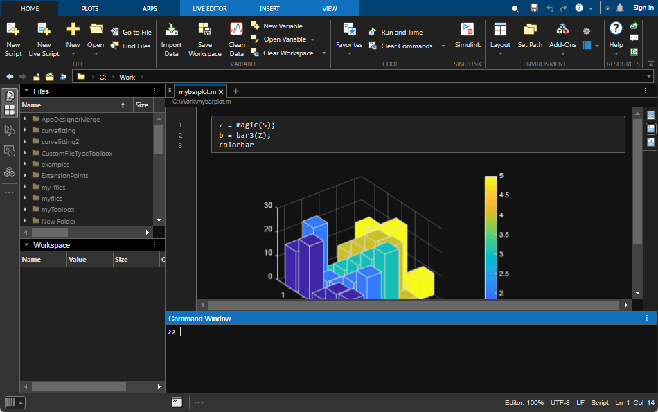
To further customize the colors of the MATLAB desktop, select MATLAB > Appearance > Colors. Then, change the colors in the Desktop tool colors, MATLAB syntax highlighting colors, and MATLAB output colors sections.
As part of this change, icons in the MATLAB Online desktop have an improved visual appearance.
For more information about changing the colors of the MATLAB desktop, see Change Desktop Colors.
Live Editor Colors: Change the text and background colors of live scripts and functions
You can change the text and background colors in the Live Editor by changing the MATLAB desktop tool colors.
To change the text and background colors:
On the Home tab, in the Environment
section, click
Preferences.
Select MATLAB > Colors
In MATLAB Online, select MATLAB > Appearance > Colors.
In the Desktop tool colors section, clear the Use system colors check box.
In MATLAB Online, the Use system colors check box is not available and this step can be skipped.
Use the Text and Background fields to change the colors. For example, select white for the text color and black for the background color.
The Live Editor automatically selects colors for titles and headings based on the selected background color. To further customize the colors of titles and headings, use settings. For more information, see matlab.fonts Settings.
Live Editor Hyperlinks: Insert hyperlinks to specific locations in separate live scripts or live functions
Use hyperlinks to navigate to a location in a separate, existing live script or function. To insert a hyperlink, select the text to link in the current file, go to the Insert tab, and click Hyperlink. Edit your display text (optional), select Location in existing document, and enter or browse for the file path. Then, select a location in the document preview that displays on the right.
For more information about inserting hyperlinks, see Format Text in the Live Editor.
Live Editor Export: Export live scripts and functions programmatically using the
export function
Use the export
function to programmatically export live scripts and functions to a standard format.
Available formats include PDF, Microsoft® Word, HTML, and LaTeX.
For example, to export the live script homework1.mlx as HTML,
type:
export("homework1.mlx","homework1.html")
Live Editor Accessibility: Interact with output in live scripts using the keyboard
You can now use keyboard shortcuts to interact with output in live scripts when output is on the right. To move focus from the code to the output display panel, press Ctrl+Shift+O. On macOS, press Option+Command+O. To activate an output, press Enter. Once an output is activated, you can scroll text using the arrow keys, navigate through hyperlinks and buttons using the Tab key, and open the context menu by pressing Shift+F10.
Live Editor Tasks: View and interact with tasks when code is hidden
When you hide code in a live script, the Live Editor now displays Live Editor tasks along with formatted text, labeled controls, and output.
To hide code, select the Hide Code button to the right of the live script or in the
View tab. Alternatively, if you are using the export
function, you can hide the code using the HideCode name-value
argument.
If a Live Editor task is configured to show only code and no controls, then the task does not display when you hide code.
Component Browser: Reorder children in App Designer or the Property Inspector
You can now drag one or more Axes object children,
Group object children, or Transform object
children sharing the same parent to reorder them in the Component Browser in App
Designer or the Property Inspector for figures.
When reordering children, use visual feedback for allowed moves. You can undo and redo the reordering of the children with Undo or Redo or the corresponding keyboard shortcuts.
Editor Python Support: View and edit Python files with syntax highlighting, auto-indenting, and delimiter matching
The Editor now displays Python® files with syntax highlighting for keywords, strings, comments, and errors. In addition, the Editor auto-indents Python files and indicates matched and mismatched delimiters such as parentheses, brackets, and braces.
Find and Replace Dialog Box: Search text in the Editor and Live Editor using regular expressions
You can use a subset of regular expressions to search for text that matches a pattern
in an open file in the Editor or Live Editor. To search using a regular expression, on
the Editor or Live Editor tab, in the
Navigate section, click
Find. Then, in the find and replace dialog box, enter
a regular expression, and select the Regular Expression button
.
For example, to find all the words in a file that contain the letter
x, enter the expression \w*x\w* and select the
Regular Expression button
.

For more information, see Find and Replace Text in Files and Go to Location.
Profiler: Access the Profiler from the Apps tab
The MATLAB Profiler is now available as an app and can be found in the MATLAB section of the apps gallery in the Apps tab.
You can still access the Profiler from the Home tab,
in the Code section, by clicking the Run and
Time button, or programmatically using the profile function.
Internationalization: UTF-8 system encoding on Windows platforms
MATLAB now uses UTF-8 as its system encoding on Windows®, completing the adoption of Unicode® across all supported platforms. MATLAB has used UTF-8 as the default encoding for MATLAB files and file I/O since R2020a.
If you see garbled characters on a Windows Server® 2019 platform, then enable the Beta: Use Unicode UTF-8 for worldwide language support option in Region Settings.
Installation Settings: Configure persistent settings for MATLAB installations
Installation-level settings provide a new layer of MATLAB configuration that lies between factory settings and personal settings. Installation settings override the factory settings for all users of a given MATLAB installation, and they are persistent across sessions.
In previous versions of MATLAB, if administrators wanted to limit RAM usage for a set of MATLAB users by lowering the ArraySizeLimit, they had to
create and distribute a script to change the personal setting for each individual user.
Starting in R2022a, the administrator can apply the change to all users of their MATLAB
installation using the installation setting for
ArraySizeLimit.
Access installation-level settings using the new
InstallationValue property of the Setting
object. Verify and clear installation settings with two new object functions,
hasInstallationValue and
clearInstallationValue, respectively.
Comparison Tool: Save results as HTML report
You can now use the Comparison Tool to publish text comparison results in an HTML report. For more details, see Compare Text Files.
Comparison Tool: Compare folders in MATLAB Online
Starting in R2022a, you can compare folders and zip files in MATLAB Online.
You can access the comparison tool from:
The MATLAB Current Folder browser context menu
The Current Project browser context menu
The MATLAB Command Window using the visdiff function
MATLAB Drive: macOS 10.15 Catalina will no longer receive updates to MATLAB Drive Connector (April 2022)
After this release, macOS 10.15 Catalina will no longer receive updates to MATLAB Drive™ Connector.
Installing later versions of MATLAB Drive Connector on macOS 10.15 Catalina will not be supported. In addition, the Connector will not automatically update to a later version when one becomes available.
Functionality being removed or changed
Live Editor figure size is bounded upon saving
Behavior change
When opening a saved live script, existing images in the output have a maximum size equivalent to the figure size upon saving. To adjust the size past this maximum limit, you can run the live script and increase the figure size.
Class Introspection: Description and
DetailedDescription properties of metaclasses contain text from
code comments
The Description and DetailedDescription
properties of these metaclasses pull content from code comments:
For user-defined classes with appropriately placed code comments, the
Description and DetailedDescription
properties of the metaclasses are populated with text pulled from those comments. For
more information on how to use code comments to store custom help text for user-defined
classes, see Custom Help Text.
Class Introspection: Access class aliases from meta.class
instance
The aliases of a class are stored in the new Aliases property of
meta.class. For more information on class
aliasing, see Creating and Managing Class Aliases.
Background Pool: See futures in the background
Starting in R2022a, you can query all queued and running futures in the background by
using the FevalQueue property of the pool. To create futures, use
parfeval and parfevalOnAll. For more
information on futures, see Future.
cancelAll Method: Cancel currently queued and running futures in
the background pool
cancelAll
cancels all futures currently queued or running in the background pool. Queued or
running futures are listed in the FevalQueue property.
Background Pool: Check the status of the background pool
Starting in R2022a, you can query to determine if the background pool is currently
running by using the Busy property of the pool. This property
indicates whether the background pool is busy, specified as true or
false. The pool is busy if there is outstanding work for the pool
to complete.
pcode Function: Create P-code files with enhanced
obfuscation
The pcode function now has the option
"-R2022a", which creates P-code files using a more complex
obfuscation algorithm. Files created with this option run only in MATLAB releases R2022a and later.
str2num Function: Restrict evaluation to basic math
expressions
str2num is implemented using the
eval function, which evaluates the input argument. Starting in
R2022a, you can set the name-value argument Evaluation to
"restricted" to restrict accepted inputs to basic math
expressions, such as 200 and 1+2i.
assert Function: Output displays which assertion threw an error
and the location in the code
When an assertion fails, the error thrown includes the specific assertion that failed and the location in the code.
| Previous Output | New Output |
|---|---|
Error using repro>checkScalarInteger Assertion failed. Error in repro (line 4) checkScalarInteger(pi) |
Error using assert Assertion failed. Error in assert_test>checkScalarInteger (line 6) assert(x == floor(x)) Error in assert_test (line 3) checkScalarInteger(pi) |
Functionality being removed or changed
Defining classes and packages: Using schema.m will not be
supported in a future release
Still runs
Support for classes and packages defined using schema.m files
will be removed in a future release. Replace existing schema-based classes with
classes defined using the classdef keyword.
dec2hex and dec2bin input types are now
restricted
Behavior change
cd no longer removes leading spaces for Windows drive letter
paths
Behavior change
Before R2022a, on Windows platforms, the cd function removed leading spaces in input
paths specifying the drive letter. Input paths containing leading spaces now cause
an error to be thrown instead. If an input path is invalid with leading spaces, then
use strip to remove the spaces before
using the cd function.
TruncateScalarObject name-value argument for
widthConstrainedDataRepresentation method renamed to
AllowTruncatedDisplayForScalar
Behavior change in future release
The name of the TruncateScalarObject name-value argument for
the widthConstrainedDataRepresentation method is now
AllowTruncatedDisplayForScalar. The functionality of the
option will not change. Support for the name
TruncateScalarObject will be removed in a future
release.
cast returns consistent output for subclass of MATLAB numeric types
Behavior change
The syntax cast(A,"like",p) now returns output consistent
with the prototype p when the data type of p
is a subclass of MATLAB numeric types.
For example, this code returns an output that has the same data type as
p:
p = matlab.lang.OnOffSwitchState.on;
x = cast(1,"like",p)x =
OnOffSwitchState enumeration
onx = 1 with data type
logical.Error reports will no longer include line number
Behavior change
Thrown error reports will no longer include the line number of where the error occurred.
Data Cleaner App: Interactively preprocess and organize column-oriented data
The new Data Cleaner app enables you to:
Access column-oriented data in the MATLAB workspace or import column-oriented data from a file.
Explore data by using the visualization, data, and summary views.
Sort by a variable, rename a variable, or remove a variable.
Retime data in a timetable, stack or unstack table variables, clean missing data, clean outlier data, smooth data, or normalize data.
Edit previously performed cleaning steps by using the Cleaning Steps panel.
Export cleaned data to the MATLAB workspace, or export code for cleaning data as a script or function.
You can open the Data Cleaner app from the MATLAB section of the apps gallery in the Apps tab.
Alternatively, enter dataCleaner in the MATLAB command window.
The Data Cleaner app currently supports cleaning only timetable data and importing only one timetable at a time.
allfinite, anynan, and
anymissing Functions: Determine if all array elements are
finite, any element is NaN, and any element is missing
Use the allfinite, anynan, and
anymissing functions to examine the elements of an input
array.
allfinite: Determine if all array elements are finite.
anynan: Determine if any array element is
NaN.
anymissing: Determine if any array element is missing.
quantile, prctile, and
iqr Functions: Calculate quantiles, percentiles, and
interquartile range
rms Function: Calculate root-mean-square value
Calculate the root-mean-square (RMS) value of input data with rms.
You can specify the dimensions to operate along and whether to include or omit
NaN values in the calculation:
Use "all" to calculate the RMS value of all elements of
the input array.
Use the dim input argument to calculate the RMS value
along one dimension.
Use the vecdim input argument to calculate the RMS
value along multiple dimensions.
Use "includenan" or "omitnan" to
include or omit NaN values in the RMS calculation.
Previously, the rms function required Signal Processing Toolbox™.
Date and Time Functions: Some Financial Toolbox functions combined with MATLAB functions
The following date and time functions from Financial Toolbox™ are combined with functions having the same names in MATLAB. Before R2022a, these Financial Toolbox functions supported serial date numbers and text timestamps as inputs,
while the MATLAB functions supported datetime arrays. Starting in
R2022a, the MATLAB functions support datetime arrays, serial date numbers,
and text timestamps as inputs. The functions are removed from Financial Toolbox.
While these functions support serial date number and text inputs, these types of
inputs are not recommended. Use datetime values as inputs
instead. The datetime data type provides flexible date and time
formats, storage out to nanosecond precision, and properties to account for time
zones and daylight saving time. To convert serial date numbers or text timestamps to
datetime values, use the datetime function.
To convert serial date numbers to datetime values, call
datetime with the ConvertFrom
name-value argument:
dt = datetime(738457,"ConvertFrom","datenum")
dt = datetime 28-Oct-2021
To convert text timestamps, call
datetime.
dt = datetime("2021-10-28")
dt = datetime 28-Oct-2021
There are no plans to remove support for serial date numbers or text timestamps from these MATLAB functions.
Date and Time Functions: Some Financial Toolbox functions moved to MATLAB
These date and time functions are removed from Financial Toolbox and moved to MATLAB:
While MATLAB supports these functions, they are not recommended because they use
serial date numbers in their calculations. The table shows recommended replacements
that either accept or return datetime values. The
datetime data type is recommended because it provides
flexible date and time formats, storage out to nanosecond precision, and properties
to account for time zones and daylight saving time.
There are no plans to remove these functions from MATLAB.
Transferred Function | Recommended Replacement |
|---|---|
|
|
|
|
|
|
|
|
|
|
|
|
|
|
|
|
matlab.datetime.compatibility.convertDatenum Function: Convert
text timestamps and serial date numbers to datetime values in a
backward-compatible way
To convert text timestamps and serial date numbers to datetime
values, use the matlab.datetime.compatibility.convertDatenum function. For backward
compatibility, this function supports the subset of datestr formats that the datenum function recognizes when it converts text timestamps without a
format specifier.
Use this function in code where you intend to return datetime
values, but to preserve compatibility you need to interpret text inputs in the same way
that datenum interprets them. This function is designed to be a
compatibility layer for function authors.
To explicitly convert serial date numbers to datetime values, use
the datetime function instead, with the
ConvertFrom name-value argument:
dt = datetime(738457,"ConvertFrom","datenum")
dt = datetime 28-Oct-2021
categorical Data Type: Use a pattern object to
specify category names that match a pattern
When you specify category names of a categorical array, you can use
a pattern
object to specify names that match a pattern.
For example, suppose you have a categorical array that has many different categories that can represent "yes" and "no". This categorical array has six values and six categories because the values in the input array are different.
C = categorical(["Y" "Yes" "Yeah" "N" "No" "Nope"])
C =
1×6 categorical array
Y Yes Yeah N No Nope
To combine all the different "yes" categories into one category and all the different
"no" categories into another category, use the mergecats function
and wildcard patterns to match the category names. The categorical array still has six
values. But it has only two categories, "yes" and
"no".
C = mergecats(C,"Y" + wildcardPattern,"yes"); C = mergecats(C,"N" + wildcardPattern,"no")
C =
1×6 categorical array
yes yes yes no no no
These functions provide support for using patterns when you specify category names:
histcounts (when you
specify the Categories argument)
iscategory (when you
specify the catnames argument)
mergecats (when you specify
the oldcats argument)
removecats (when you
specify the oldcats argument)
reordercats (when you
specify the neworder argument)
table and timetable Data Types: Use a
pattern object to specify row, variable, and property names that
match a pattern
When you specify rows, variables, or properties of a table or timetable, you can use a
pattern
object to specify names that match a pattern.
You can use patterns when you subscript into a table by row names and variable names, or when you subscript into a timetable by variable names.
For example, read a table into MATLAB.
T = readtable("outages.csv","TextType","string")
T =
1468×6 table
Region OutageTime Loss Customers RestorationTime Cause
___________ ________________ ______ __________ ________________ __________________
"SouthWest" 2002-02-01 12:18 458.98 1.8202e+06 2002-02-07 16:50 "winter storm"
"SouthEast" 2003-01-23 00:49 530.14 2.1204e+05 NaT "winter storm"
"SouthEast" 2003-02-07 21:15 289.4 1.4294e+05 2003-02-17 08:14 "winter storm"
: : : : : :
To subscript into the table and select all variables whose names end with
"Time", use a wildcard pattern.
T2 = T(:,wildcardPattern + "Time")
T2 =
1468×2 table
OutageTime RestorationTime
________________ ________________
2002-02-01 12:18 2002-02-07 16:50
2003-01-23 00:49 NaT
2003-02-07 21:15 2003-02-17 08:14
: :
These functions provide support for using patterns when you specify variables by name:
This function provides support for using patterns when you specify properties by name:
Data Preprocessing Functions: Append transformed variables to input data using the
ReplaceValues name-value argument
When you preprocess tables and timetables, you can now append variables containing the
transformed values to the input table. Set the ReplaceValues
name-value argument to false for these functions:
Data Preprocessing Functions: Return table with logical values using the
OutputFormat name-value argument
When you preprocess tables and timetables, you can now output a table or timetable
containing logical values instead of a logical array. Set the
OutputFormat name-value argument to "tabular"
for these functions:
ismissing, rmmissing, and
groupsummary Functions: Accept data types with no standard
missing value
The ismissing syntax
ismissing(A) now returns logical 0
(false) when the input data type has no default definition of a
standard missing value.
rmmissing and the
nummissing and nnz methods of groupsummary no longer error for input data types with no default
definition of a standard missing value.
An example of code that used to error but now executes is:
A = [struct struct struct]; TF = ismissing(A)
TF =
1x3 logical array
0 0 0Some input types that used to throw an error now execute. If your code relies on
the errors that MATLAB threw for those inputs, such as within a try/catch
block, then your code may no longer catch those errors.
Functionality being removed or changed
Plot a variable multiple times in a stacked plot
Behavior change
You can now display the same table or timetable variable multiple times when you
call the stackedplot function. In previous releases, specifying a variable
more than once results in an error.
For example, create a timetable from the outages.csv file. Then
plot the RestorationTime variable under each of the other
variables that you specify.
tbl = readtimetable("outages.csv"); tbl = sortrows(tbl); stackedplot(tbl,["Loss","RestorationTime","Customers","RestorationTime"])
Live Editor tasks for arrays, tables, and timetables do not run automatically if inputs have more than 1 million elements
Behavior change
Many Live Editor tasks for arrays, tables, and timetables do not run automatically if inputs have more than 1 million elements. In previous releases, these tasks run automatically for input arrays, tables, and timetables of any size. If the inputs have a large number of elements, then the code generated by these tasks can take a noticeable amount of time to run (more than a few seconds).
This change in behavior affects these tasks:
Live Editor tasks for preprocessing data do not run automatically if inputs have more than 1 million elements
Behavior change
Many Live Editor tasks for preprocessing data do not run automatically if inputs have more than 1 million elements. In previous releases, these tasks run automatically for input data of any size. If the inputs have a large number of elements, then the code generated by these tasks can take a noticeable amount of time to run (more than a few seconds).
This change in behavior affects these tasks:
Parquet: Read Parquet file data more efficiently using rowfilter
to conditionally filter rows
Conditionally filter and read data faster (Predicate Pushdown) from Parquet files when
using parquetread and parquetDatastore. You can create conditions for filtering by using the
rowfilter function, matlab.io.RowFilter object, and RowFilter name-value
argument. Due to its metadata-accelerated processing, the rowfilter
workflow is the recommended approach for filtering Parquet data to import.
Parquet: Determine and define row groups in Parquet file data
A Parquet file can store a range of rows as a distinct row group for increased
granularity and targeted analysis. parquetread uses the
RowGroups name-value argument to determine row groups while
reading Parquet file data. parquetwrite uses the
RowGroupHeights name-value argument to define row groups while
writing Parquet file data.
Parquet: Convert, import, and export nested data structures
Use parquetread to import nested
Parquet file data with:
LogicalType as LIST.
LogicalType as NONE and
PhysicalType as either BYTE_ARRAY
or FIXED_LEN_BYTE_ARRAY.
The parquetread function converts and imports these
data structures as cell arrays.
Use parquetwrite to export nested
cell arrays as LIST arrays. Nested data is beneficial to working with irregularly
structured data such as jagged arrays.
writelines Function: Write plain text to a file
Use the writelines function to write a string array or a cell array of character
vectors as plain text to a file. The writelines function is the
writing equivalent of the readlines function.
Reading Online Data: Use web options when reading files over HTTP and HTTPS
Read files over HTTP and HTTPS using the weboptions function and specifying the WebOptions
name-value argument with these functions:
Opus Files: Work with Opus (.opus) audio files.
Use audioread, audiowrite, and audioinfo to read, write, and analyze Ogg Opus audio files.
HDF5 Interface: Write datasets using dynamically loaded filters
You can read and write HDF5 datasets using dynamically loaded filters with both the high-level and low-level interfaces. For details, see Import HDF5 Files and Export to HDF5 Files.
The h5create function introduces two name-value arguments,
CustomFilterID and CustomFilterParameters, to enable compression using dynamically loaded
filters.
NetCDF Interface: Enable byte-range reading of remote datasets
You can now use the existing high-level and low-level interfaces for read-only access to remote datasets using the HTTP byte-range capability. The latter assumes that the remote server supports byte-range access.
NetCDF Interface: Read and write variable length array data types
(NC_VLEN)
You can now use the existing high-level functions to read variable length array data
types (NC_VLEN) from NetCDF-4 files. You can read and write
NC_VLEN types using low-level functions.
Use these additional low-level functions to create NC_VLEN types
and retrieve information about them:
Scientific File Format Libraries: NetCDF library is upgraded
The NetCDF library is upgraded to version 4.8.1.
Hardware Manager App: Discover and connect to your hardware from MATLAB
The new Hardware Manager app allows you to discover and connect to your hardware from MATLAB by providing access to the necessary add-ons and apps. For more information, see Get Started with Hardware Manager.
TCP/IP Client Interface: Specify transfer delay options
You can now enable or disable a transfer delay to allow delayed acknowledgement from
the connected server for tcpclient objects and in the TCP/IP
Explorer app. The transfer delay is enabled by default. Enabling the delay
turns on Nagle's algorithm, which causes the client to collect small segments of
outstanding data and send them in a single packet when acknowledgement (ACK) arrives
from the server. Disabling it turns off Nagle's algorithm, which immediately sends data
to the network.
For the tcpclient interface, you can set the
EnableTransferDelay property as a name-value argument during
object creation. For TCP/IP Explorer, you can select Transfer
Delay options during connection configuration.
For more information about this functionality, see EnableTransferDelay and Configure Connection in TCP/IP Explorer.
Functionality being removed or changed
seriallist function will be removed
Warns
seriallist will be removed. Use
serialportlist instead. For more information about updating
your code to use the recommended functionality, see Transition Your Code to serialport Interface.
serial function will be removed
Warns
serial and its object properties will be removed. Use
serialport and its properties instead.
This example shows how to connect to a serial port device using the recommended functionality.
| Functionality | Use Instead |
|---|---|
s = serial("COM1");
s.BaudRate = 115200;
fopen(s) |
s = serialport("COM1",115200); |
For more information about updating your code to use the recommended
functionality, see Transition Your Code to serialport Interface.
MATLAB Variable Editor: timeseries will no longer be
supported
Warns
Viewing timeseries objects using the MATLAB Variable Editor will no longer be supported. To view time-indexed data
in the Variable Editor, use timetable instead.
pagemldivide, pagemrdivide, and pageinv Functions:
Solve linear equations and calculate matrix inverses using pages of N-D arrays
Use the pagemldivide, pagemrdivide, and
pageinv functions to perform linear algebra operations on the
pages of N-D arrays. In this context, the N-D array is treated as a container for
several 2-D matrices.
pagemldivide and pagemrdivide: Solve linear equations using the pages of N-D
arrays.
pageinv: Calculate the matrix inverse of the pages of an N-D
array.
tensorprod Function: Calculate tensor products between two
arrays
Use the tensorprod function to calculate tensor products between two N-D arrays.
You can perform an inner product, outer product, or a combination of the two by
specifying a subset of dimensions to contract (multiply and sum) with each other.
round Function: Control tiebreak behavior
The round function has a new
TieBreaker name-value argument to specify how to break ties. You
can now specify to round ties away from zero, towards zero, to the nearest even or odd
integer, or towards positive or negative infinity.
Starting in R2022a, the round function always rounds ties (that
are within roundoff errors) away from zero by default. In previous releases, the
round function sometimes returns inconsistent results, where
ties are rounded towards zero by default.
null and orth Functions: Specify tolerance
to treat singular values below a threshold as zero
norm Function: Frobenius norm calculations support N-D
arrays
Frobenius norm calculations of the form norm(X,"fro") now support
N-D arrays. See norm for more information.
equilibrate Function: Specify output format of
factorization
equilibrate now has an option with values of "vector"
or "matrix" to specify whether the output arguments are returned as
vectors or matrices. For large factorizations, returning the outputs as vectors can save
memory and improve efficiency.
rand, randi, and randn
Functions: Support for complex input and RandStream object with the
"like" syntax
The rand, randi, and randn functions now support complex input
and a RandStream object for the "like"
syntax.
For example, you can use X = rand(m,n,"like",p) to create an
m-by-n array of random numbers of the same
data type and complexity (real or complex) as p. You can also use
X = rand(s,m,n,"like",p) to generate random numbers like
p from the random number stream s
(RandStream object) instead of the default global stream.
eps, flintmax, intmax,
intmin, realmax, and
realmin Functions: Use "like" syntax to return
scalars based on prototype object
The eps, flintmax, intmax, intmin, realmax, and realmin functions now accept the "like" syntax to
return scalars based on a prototype object.
For example, you can use f = realmax("like",p) to return the
largest finite floating-point number with the same data type, sparsity, and complexity
(real or complex) as the floating-point variable p.
Functionality being removed or changed
One-output qr syntax always returns upper-triangular
factor
Behavior change
The syntax R = qr(A) always returns R as an
upper-triangular matrix, regardless of whether A is full or
sparse. Previously, for full A, the one-output syntax returned an
R matrix with intermediate data used in the calculation
located in the lower triangular portion of the matrix. See qr for more information.
mldivide no longer uses LDL factorization for full
matrices
Behavior change
mldivide no longer uses an LDL
factorization for full matrices that are Hermitian indefinite. Instead, the LU
factorization is used for these matrices.
Plotting Table Data: Create line plots by passing tables directly to plotting functions
Create plots by passing a table directly to any of these functions: plot,
plot3, loglog, semilogx, semilogy, and polarplot. When you specify your data as
a table, Cartesian axis labels and the legend (if present) are automatically labeled
using the table variable names.
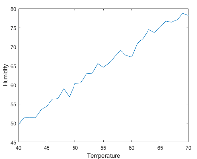
For example, create a table with the variables Temperature and
Humidity. Pass the table to the plot
function as the first argument, and specify the variables you want to plot.
Temperature = (40:70)'; Humidity = (50:80)' + randn(31,1); T = table(Temperature,Humidity); plot(T,"Humidity","Temperature")
Data Tips: View table variable names as row labels
When plotting tabular data, the default row labels of data tips created interactively
or with the datatip
function are the names of the table variables associated with the data point.
For example, create a table using the sample file patients.xls.
Then, plot the Systolic, Diastolic, and
Weight variables in a bubble chart. A data tip created with
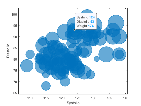
datatip(b) displays three rows. The row labels are "Systolic",
"Diastolic", and "Weight".
tbl = readtable("patients.xls"); b = bubblechart(tbl,"Systolic","Diastolic","Weight"); datatip(b);
Data Tips: View visual property values for scatter plots and bubble charts
For scatter plots and bubble charts, data tips created interactively or with the
datatip
function include by default rows for visual properties such as size, color, or
transparency that are specified with vector data.
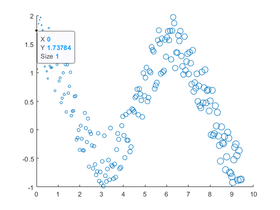
For example, create a scatter plot of random data and define the marker sizes as
vector sz. A data tip created with datatip(s)
displays three rows: X, Y, and
Size. The Size row in the data tip displays
the marker size specified by sz for the associated data point.
x = linspace(0,3*pi,200); y = cos(x) + rand(1,200); sz = linspace(1,100,200); s = scatter(x,y,sz); datatip(s);
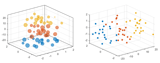
Bubble Charts and 3-D Scatter Plots: Plot multiple data sets at once
The bubblechart, bubblechart3, polarbubblechart, and scatter3 functions now accept the same combinations of matrices and
vectors as the plot function does. As a result, you can visualize multiple data sets at
once rather than using the hold function between plotting commands.
fontname and fontsize Functions: Specify the
font and font size for graphics objects
Use the fontname
and fontsize
functions to modify the fonts displayed with graphics objects such as figures, axes,
legends, tiled chart layouts, standalone visualizations, and UI components. MATLAB applies your changes to the specified object and all the objects it
contains. For example, if you change the font on a figure, all the axes, annotations,
and UI components within the figure use the new font.
exportgraphics Function: Create animated GIF files
Create animated GIF files by calling the exportgraphics function multiple times with the
Append name-value argument.
Annotation Graphics Objects: Change the annotation rotation angle with the
Rotation property
For text box, rectangle, and ellipse annotation objects, rotate the annotation a
specified number of degrees by using the Rotation property. The
anchor point for rotation is the location specified by the first two elements of the
Position property, so the Position property is
unaffected by rotation.
For more information, see TextBox Properties, Rectangle Properties, and Ellipse Properties.
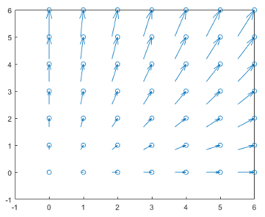
Quiver Plots: Align the heads, centers, or tails of arrows with data points
Set the Alignment property of a Quiver object
to control how the arrows align with the data points. Valid values are
"head", "center", and
"tail". For example, plot a grid of vectors with the arrow heads
positioned at the data points. Specify a marker symbol to show the locations of the data points.
[X,Y] = meshgrid(0:6,0:6); U = 0.25*X; V = 0.5*Y; quiver(X,Y,U,V,"Alignment","head","Marker","o")
view Function: Change the view on multiple axes
simultaneously
Change the view of multiple axes objects at the same time by passing an array of axes
objects to the view function.
rendererinfo Function: Get renderer information without specifying
the axes
Call the rendererinfo function without any arguments to query the default
graphics renderer information. This new syntax allows you to call the
rendererinfo function in a way that is consistent with the
opengl syntax. Since R2019a, the
rendererinfo function has been recommended instead of the
opengl function for querying the renderer.
linkaxes Function: Synchronize axes in all dimensions by
default
The linkaxes function now supports 3-D
Cartesian axes and synchronizes the x-axis,
y-axis, and z-axis limits by default. The
supported values of the dimension input argument are now
'xyz' (default), 'x', 'y',
'z', 'xy', 'xz',
'yz', and 'off'.
Before R2022a, linkaxes supported only 2-D Cartesian axes and
synchronized the x-axis and y-axis limits by
default.
cameratoolbar Function: Syntax support for figures created with
the uifigure function
Syntaxes of the cameratoolbar function that do not
directly make the toolbar visible are now supported by figures created with the
uifigure function.
Callbacks in Live Editor: Create callbacks for figures in the Live Editor
You can now create callbacks for figures created in the Live Editor. The callback workflow supports optional source and event-data parameters.
Keyboard-based callback properties and anonymous function callbacks using
Figure objects from the MATLAB workspace are not currently
supported in the Live Editor.
To define and execute a figure callback in the Live Editor, use one of these techniques:
Create a figure callback and pass source and event data as parameters in the callback.
Create a figure callback and do not pass source or event data as a parameter in the callback.
Create a callback that includes a function for identifying a graphics object,
such as gca or findobj.
For example, define a callback function called colorchangeCallback.
With the colorchangeCallback function on the MATLAB path, use the @ operator to assign the function handle
to the WindowButtonDownFcn property of the figure
fig.
fig = figure; axis([-4 4 -4 4]); plot(1:10) fig.WindowButtonDownFcn = @(src,eventdata)colorchangeCallback(src);
Define the callback and set the Color property for the
Axes object in the figure:
function colorchangeCallback(f,~) % Change the axes color on button down ax = f.Children; ax.Color = rand(1,3); end
For more information, see Callbacks in Live Editor.
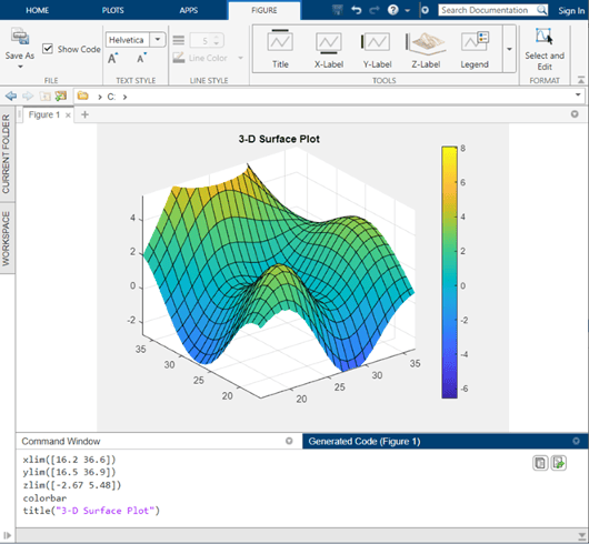
Figure Code: Generate code for figure interactions in MATLAB Online
When you modify a figure in MATLAB Online using the Figure tab, MATLAB generates code that you can view, copy, and export. To view the generated code, select Show Code in the File section of the Figure tab. MATLAB generates code for these actions:
Adding a title, axis label, legend, color bar, grid, or annotation
Changing the text or line style
Using the pan, zoom, rotate, or data tip interactions
MATLAB does not currently generate code for the Select and Edit option in the Figure tab.
For example, you can create a surface plot with surf(peaks). Then,
interactively add a title and colorbar, zoom into the axes, and view generated code.
Functionality being removed or changed
Polar axes display angle values with degree symbols
Behavior change
Polar axes now display tick values in degrees with degree symbols when the
ThetaAxisUnits property is set to
"degrees". For example, create a polar plot. By default, the
theta-axis displays the tick values with degree
symbols.
theta = 0:0.01:2*pi; rho = sin(2*theta).*cos(2*theta); polarplot(theta,rho)
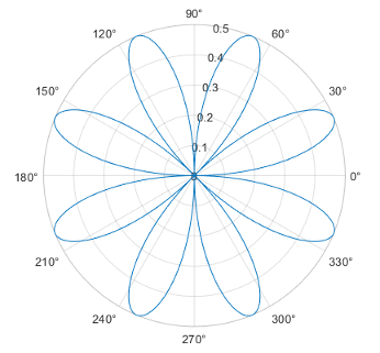
This change clarifies which units are being used for the theta
tick values. You can use the ThetaAxisUnits property to display
the tick values in degrees or radians. To remove the degree symbols, change the tick
label format for the theta-axis:
pax = gca;
pax.ThetaAxis.TickLabelFormat = "%g";The caxis function is not
recommended
Still runs
The caxis function is no longer recommended. However, the
function continues to work, and there are no plans to remove it at this time.
To update your code, call the clim
function instead. It accepts the same input arguments and returns the same output as
the caxis function.
The im2java function will be removed
Still runs
im2java will be removed in a
future release. There is no replacement for this function.
The Plot Catalog tool will be removed
Still runs
The Plot Catalog tool will be removed in a future release. Instead, to interactively create and explore visualizations for your data, use the Plots tab in the MATLAB Toolstrip or the Create Plot task in the Live Editor.
For more information about visualizations, see Types of MATLAB Plots or toolbox-specific documentation.
The opengl function will be removed
Still runs
The opengl function will be removed in a future release.
To query the renderer, use the rendererinfo function instead of the
opengl function.
Changing the renderer with the opengl function
will no longer be necessary when the function is removed.
The renderer startup options will be removed
Still runs
In a future release, the MATLAB startup options for selecting the graphics renderer will be removed. Specifically, these startup scenarios will no longer be available:
matlab -softwareopengl
matlab -nosoftwareopengl
matlab -softwareopenglmesa
matlab -noopengl
It will no longer be necessary to specify the renderer when these options are removed.
The
Renderer property of figures will have no effect
Behavior change in future release
The Renderer and RendererMode properties
of figures will have no effect in a future release. It will no longer be necessary
to change the renderer when these properties are disabled.
The FontSmoothing property will have no effect
Behavior change in future release
The FontSmoothing property for all types of axes, rulers,
geographic scales, and text objects will have no effect in a future release. Font
smoothing will be enabled regardless of the value of the property.
Some plot tools functions will redirect to the Figure Toolstrip and Property Inspector
Behavior change in future release
Calling these plot tools functions will open a configuration of the Figure Toolstrip and Property Inspector. For more information, see the Version History section in the documentation for each function.
Currently, calling plot tools functions opens the Figure Palette, Plot Browser, and Property Editor.
uistyle Function: Add icons and format text in table cells and
tree nodes
You can now create styles for table and tree UI components that specify an icon and a
text interpreter using the uistyle
function.
Specify the Icon property of the style object to add
icons to table cells and tree nodes.
Specify the IconAlignment property of the style object to
modify where the icon appears in relation to the text in table cells.
Specify the Interpreter property of the style object to
format text or add links using HTML markup, or to add equations using TeX or
LaTeX markup to table cells and tree nodes.
Specify the HorizontalClipping property of the style
object to control whether long text is clipped on the left or the right in table
cells and tree nodes.
Add a style to a UI component using the addStyle
function.
For example, this code creates two styles, one that specifies an icon and one that specifies the text interpreter as TeX, and applies the styles to columns of a table.
T = table(["x^2";"3x^3+1"],["Success";"Success"]); fig = uifigure(Position=[500 500 300 160]); t = uitable(fig,Position=[10 10 250 140],Data=T); s1 = uistyle(Interpreter="tex"); s2 = uistyle(Icon="success",IconAlignment="right"); addStyle(t,s1,column=1) addStyle(t,s2,column=2)

uitable Function: Rearrange columns of table UI components
interactively
You can specify the ability to interactively rearrange table columns in an app by
using the ColumnRearrangeable property. In a table UI component
with the ColumnRearrangeable value set to 'on',
rearrange table columns in the app by clicking and dragging the column header.
In App Designer and apps created using the uifigure function, you
can program an app to respond when a user rearranges table columns by creating a
DisplayDataChangedFcn callback function.
For more information, see Table Properties.
focus Function: Give keyboard focus to UI components
programmatically
Use the focus
function to programmatically give focus to keyboard-focusable UI components. When a UI
component is focused, it is displayed with a blue focus ring, and app users can interact
with the component using the keyboard.
isInScrollView Function: Determine if a component is visible in
a scrollable container
Use the isInScrollView function to programmatically identify which components
are visible given the size and scroll location of a scrollable container. For example,
you can determine which axes are visible inside a scrollable figure window and then
update the data only for those axes.
uigridlayout Function: Resize table, list box, and image UI
components to fit content
Grid layout managers with row heights or column widths of 'fit' now
resize to fit the contents of table, list box, and image UI components.
For example, when you create a table UI component inside a grid layout manager with a
row height or column width of 'fit', the height of the row or the
width of the column resizes to fit the data in the
table.
fig = uifigure(Position=[680 558 300 170]);
gl = uigridlayout(fig);
gl.RowHeight = {'fit'};
gl.ColumnWidth = {'fit'};
tbl = uitable(gl,Data=rand(3));
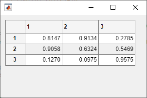
In R2021b, grid layout managers with row heights or column widths of
'fit' scaled to a fixed size when the row or column contained
a table, list box, or image UI component.
Table UI component — Row height and column width previously resized to 300 pixels.
List box UI component — Row height previously resized to display at most four items. The exact pixel value to display four items might vary depending on your settings.
Image UI component — Row height and column width previously resized to 100 pixels.
To display a table, list box, or image at its size in a release before R2022a, set
the corresponding elements of the RowHeight and
ColumnWidth properties of the
GridLayout object to their respective fixed sizes.
Live Editor Tasks: Develop your own Live Editor tasks for use in live scripts and functions
Live Editor tasks are simple point-and-click interfaces that can be embedded into a live script. Tasks represent a series of MATLAB commands that are automatically generated as users explore parameters.
You can develop your own custom Live Editor tasks by creating a subclass of the
LiveTask base class. Develop tasks to perform your own specific set
of operations within a live script.
For more information, see Live Editor Task Development Overview.
Custom UI Components: Interactively create custom UI components in App Designer
Use App Designer to interactively build your own UI components. Open a new blank custom UI component in App Designer, lay out the component by combining existing MATLAB UI components or graphics objects, and configure the component interface by creating public properties and public callbacks that can be set when the component is used in an app.
Creating a custom UI component has these benefits:
Modularization — Separate the display of large apps into independent, maintainable pieces.
Reusability — Provide a convenient interface for adding and customizing similar components in apps.
Flexibility — Extend the appearance and behavior of existing UI components.
For more information, see Create a Simple Custom UI Component in App Designer.
App Designer: Modify tab focus order of components
You can view and modify the order in which components in your app receive keyboard focus when the app user presses Tab. First, sort and filter the Component Browser by tab order by selecting Sort & Filter by Tab Order from the drop-down list labeled View. The Component Browser lists only the components in the app that can have focus, in the order of focus. You can then change the tab order of the components by clicking and dragging the component names in the Component Browser.
Alternatively, App Designer can automatically apply a left-to-right and then top-to-bottom tab focus order for components in a container. Right-click the name of the container in the Component Browser and select Apply Auto Tab Order.
App Designer: Specify error handling options and navigate from error messages when debugging an app
To specify error handling options when debugging code in App Designer, configure the
Run button by clicking Run
. You can choose to pause code execution when an error
occurs, when a warning occurs, or when a NaN or
Inf value is returned.
Additionally, error messages in App Designer now contain links to relevant files and functions. Use these links to navigate more easily to the documentation or to line numbers in your code when debugging your apps.
App Designer: Manage image files in your app with an improved workflow
When you specify image data for your app, such as the image source of an image component or the icon of a button, select an image that is in the same folder as the MLAPP file or one of its subfolders. The image will then load whenever the app is opened or run without it needing to be on the MATLAB path. Alternatively, you can continue to use images in any location by adding the image files to the MATLAB path.
App Designer: Convert components in a grid layout manager to use pixel-based positioning
You can delete a grid layout manager and convert the components in the grid to use pixel-based positioning. To use pixel-based positioning when you were previously using a grid layout manager, right-click the container with the grid layout manager in the canvas, and select Remove Grid Layout.
For more information, see Use Grid Layout Managers in App Designer.
App Designer: Use App Designer in most modern web browsers in MATLAB Online
You can now use App Designer in MATLAB Online with the current versions of Mozilla® Firefox®, Apple Safari, and Microsoft Edge®, in addition to Google Chrome®.
App Designer: Customize design environment layout
You can now customize the locations of the side panels and tabs in the App Designer design environment.
To change the location of side panels such as the Component Library and the Component Browser, click the panel header and drag it to a new location in the App Designer environment. To change the location of your open tabs to display on the left, right, or bottom of the working area, right-click the tab bar and select Tab Position.
Your changes to the design environment layout now persist even after you close and reopen App Designer.
Comparison Tool: Compare and merge app files in MATLAB Online
Compare and merge two versions of an app file in MATLAB
Online using the Comparison Tool. To open the Comparison Tool, click
Compare in the Designer tab of the App
Designer Toolstrip.
For more information, see Compare and Merge Apps.
Functionality being removed or changed
RearrangeableColumns property of table UI components is not
recommended
Still runs
Starting in R2022a, using the RearrangeableColumns property
to specify the ability to rearrange columns in a table UI component is not
recommended. Use the ColumnRearrangeable property instead. The
new property can have the same values as the old one.
There are no plans to remove support for the
RearrangeableColumns property at this time. However, the
RearrangeableColumns property no longer appears in the list
returned by calling the get function on a table UI
component.
UIAxes content is not displayed in App Designer Design View
when the component is off the canvas
Behavior change
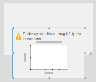
When creating an app with a UIAxes component in App Designer,
the UIAxes component content is not displayed in Design
View when the component is partially or fully off the canvas.
Instead, the UIAxes component is shown as a placeholder image. To
see the content of the component, drag it fully onto the canvas.
You can still modify properties of the UIAxes component when it
is off the canvas, but you will not be able to see a visual reflection of those
changes in Design View until the component is dragged onto the
canvas.
ComponentContainer class assigns a parent before executing the
setup method
Behavior change
When you create an instance of a custom UI component created using the matlab.ui.componentcontainer.ComponentContainer class, the class now
assigns the component parent before executing the setup method. As
a result, you might see unexpected behavior if your setup method
creates underlying UI components that can be parented to either a figure created
using the figure function or a figure created the
uifigure function, such as panels, tab groups, or button
groups.
To update your class code, when you create such a component, specify the property
value explicitly for any property where the default value differs depending on the
parent. For example, to create a panel in your custom component that is sized using
normalized units, specify Units as
"normalized" before setting the Position
property.
ButtonDownFcn callback cannot be interactively assigned for
custom UI components in App Designer
Behavior change
Starting in R2022a, when you use a custom UI component in an app in App Designer,
you cannot interactively assign a ButtonDownFcn callback to the
component. If you have an existing App Designer app that contains a custom UI
component with a ButtonDownFcn callback that you assigned
interactively, opening the app in R2022a disconnects the callback from the
component. To reassign the callback to the component, follow these steps:
If your app does not contain a StartupFcn callback,
right-click the app node from the top of the Component
Browser hierarchy and select Callbacks > Add StartupFcn Callback.
In Code View, in the
startupFcn function, add this code to assign the
appropriate ButtonDownFcn callback
programmatically:
app.CustomUIComponentName.ButtonDownFcn = ...
@(src,event)CallbackFunctionName(app,event);For example, if your app contains a custom UI component named
app.IPAddress with a
ButtonDownFcn callback named
IPAddressButtonDown, add this code to the
startupFcn function of your app:
app.IPAddress.ButtonDownFcn = @(src,event)IPAddressButtonDown(app,event);
table Data Type Indexing: Improved performance when subscripting
with dot notation or multiple levels of indexing
table subscripting when using dot notation is significantly faster
in R2022a than in R2021b. Also, subscripting with multiple levels of indexing is
faster.
For example, when you use dot notation to refer to a table variable with 106 elements, performance in R2022a is more than 4x faster than in R2021b.
function timingTest() t = table(zeros(1e6,1), ones(1e6,1), nan(1e6,1)); indices = 1:1e5; tic; % Refer to variable using dot notation for i = indices x = t.Var1; end toc end
The approximate execution times are:
R2021b: 1.55 s
R2022a: 0.36 s
Similarly, when you use dot notation to assign an array to a table variable with 106 elements, performance in R2022a is about 3x faster than in R2021b.
function timingTest() t = table(zeros(1e6,1), ones(1e6,1), nan(1e6,1)); indices = 1:1e5; x = randi(1e6,1e6,1); tic; % Assign to variable using dot notation for i = indices t.Var1 = x; end toc end
The approximate execution times are:
R2021b: 2.15 s
R2022a: 0.72 s
Also, when you use dot notation and parentheses to assign individual values to elements of a table variable, performance in R2022a is more than 4x faster than in R2021b.
function timingTest() t = table(zeros(1e6,1), ones(1e6,1), nan(1e6,1)); indices = randi(1e6,1,1e5); tic; % Assign to elements using dot notation and parentheses for i = indices t.Var1(i) = rand; end toc end
The approximate execution times are:
R2021b: 5.08 s
R2022a: 1.20 s
The code was timed on a Windows 10, Intel® Xeon CPU W-2133 @ 3.60 GHz test system by calling each version of the
timingTest function.
Classes: Improved performance for static methods, constant property access, and package functions in scripts
The overhead times for these three actions when performed in scripts are reduced:
Executing a package function
Executing a static method
Accessing a constant property
The overhead times for these actions in a script are now comparable with the times of execution in a function, and the overheads are small enough that they can generally be ignored for performance considerations.
This code performs each of these actions 1,000,000 times. (The code called in each loop is shown at the end of this note.)
tic; for j = 1:1000000 out = pkg1.pkg2.packageFunction(2); end toc; tic; for j = 1:1000000 out = MyClass.staticMethod(1); end toc; tic; for j = 1:1000000 out = pkg1.PackageClass.constantProperty; end toc;
The approximate times to complete each loop are:
R2021b:
Package function: 8.4 s
Static method: 7.8 s
Constant property access: 32 s
R2022a:
Package function: 0.04 s (210x faster)
Static method: 0.031 s (252x faster)
Constant property access: 0.039 s (821x faster)
The code was timed on a Windows 10, Intel Xeon® CPU W-2133 @ 3.60 GHz test system.
For use with the test code, PackageClass must be in folder
+pkg1, and packageFunction must be in folder
+pkg1/+pkg2.
function out = packageFunction(in) out = in; end classdef MyClass methods (Static) function out = staticMethod(in) out = in; end end end classdef PackageClass properties (Constant) constantProperty = 3; end end
try Block: Improved performance when statements run
error-free
The try block shows improved performance
when the statements within the block run error-free. For example, this code is
approximately 6x faster than in the previous release:
function testTryPerformance x = 1; for i = 1:1e8 try x = x * i; catch warning("Assignment was not successful.") x = 1; end end end
The approximate execution times are:
R2021b: 2.3 s
R2022a: 0.4 s
The code was timed on a Windows 10, Intel
Xeon CPU E5-1650 v4 @ 3.60 GHz test system using the timeit
function:
timeit(@testTryPerformance)
Python Data Type Conversion: Improved performance when converting between Python and MATLAB data types in out-of-process mode
When you run Python code out of process, conversions between Python data types and MATLAB data types show improved performance.
The timingPythonList function converts a Python
list object to a MATLAB cell array. This code is about 118x faster than in the previous
release:
function timingPythonList l = py.list(['MATLAB','R',2022,'a','and',1.2,10^2, ... 2021,12,25,'2021','12','25','and', ... 2021,12,25,'2021','12','25']); tic ml = cell(l); toc end
The approximate execution times are:
R2021b: 1.18 s
R2022a: 0.01 s
The timingPythonDict function converts a Python
dictionary object to a MATLAB structure. This code is about 57.9x faster than in the previous
release:
function timingPythonDict d = py.dict(pyargs('a',1,'b',2,'c',3,'d',4,'e',5, ... 'f',6,'g',7,'h',8,'i',9,'j',10,'k',11,'l',12, ... 'm',13,'n',14,'o',15,'p',16,'q',17,'r',18, ... 's',19,'t',20)); tic ms = struct(d); toc end
The approximate execution times are:
R2021b: 0.521 s
R2022a: 0.009 s
The timingDataTransfer function converts an array with
108 elements from a MATLAB
double array to a Python
memoryview object and then back to a MATLAB
double array. This code is about 10x faster when
converting from MATLAB to Python and approximately 11x faster when converting from Python to MATLAB than in the previous release:
function timingDataTransfer data = rand(100,10^6); tic pydata = py.memoryview(data); toc tic mdata = double(pydata); toc end
The approximate execution times for converting the MATLAB
double array to the Python
memoryview object are:
R2021b: 4.0 s
R2022a: 0.4 s
The approximate execution times for converting the Python
memoryview object to the MATLAB
double array are:
R2021b: 7.7 s
R2022a: 0.7 s
All of the code was timed on a Windows 10, Intel Core® i7-10510U CPU @ 1.80 GHz 2.30 GHz test system by using Python 3.9 in out-of-process mode and calling the
timingPythonList, timingPythonDict, and
timingDataTransfer functions.
MATLAB Engine API for Python: Improved performance with large multidimensional arrays in Python
The Python multidimensional array component used by the MATLAB Engine API for Python shows improved performance when:
Converting data from Python sequences to the data types defined by the
matlab module
Transferring data back and forth between Python and MATLAB
In both cases, the improvement is noticeable when operating on arrays with at least 10 elements. When transferring data back and forth, the improvement increases as the size of the array increases.
For example, this Python code measures the execution times of two operations:
Converting a Python array of size 108 to a MATLAB
double array
Summing the elements of the MATLAB array using the MATLAB engine
The first operation is about 12x faster than in the previous release, and the second operation is about 110x faster than in the previous release:
import random
import time
import matlab.engine
eng = matlab.engine.start_matlab()
rand_array = [random.random() for i in range(10**8)]
s0 = time.perf_counter()
array_md = matlab.double(rand_array,size=(1, 10**8))
s1 = time.perf_counter() - s0
print('conversion to matlab.double(): {} seconds'.format(s1))
s0 = time.perf_counter()
sum_of_elems = eng.sum(array_md,1)
s1 = time.perf_counter() - s0
print('sum(): {} seconds'.format(s1))
The approximate execution times for the first operation are:
R2021b: 42 s
R2022a: 3.6 s
The approximate execution times for the second operation are:
R2021b: 210 s
R2022a: 1.9 s
The code was timed on a Windows 10, Intel
Xeon CPU E5-1650 v4 @ 3.60 GHz test system by using Python
perf_counter() statements.
Matrix multiplication: Improved performance when multiplying sparse and full matrices
Matrix multiplication shows improved performance when:
One of the operands is a sparse matrix, and the other is a full matrix.
The sparse operand has at least 50,000 nonzero elements.
The full operand has at least 32 columns (or at least 32 rows when transposed).
The performance improvement arises from added support for multithreading in the operation, and therefore the speedup improves as the matrix size and number of nonzero elements increase.
For example, multiplying a 102,400-by-102,400 sparse matrix with a 102,400-by-128 full matrix on a machine with 6 physical cores is about 2.7x faster than in the previous release.
function timingSparseDenseMult A = delsq(numgrid('S',322)); B = rand(size(A,2),128); tic for k = 1:10 C = A*B; end toc end
The approximate execution times are:
R2021b: 0.8 s
R2022a: 0.3 s
The code was timed on a Windows 10, Intel
Xeon CPU W-2133 @ 3.60 GHz test system by calling the
timingSparseDenseMult function.
inv Function: Improved performance when inverting large
triangular matrices
The inv function shows improved performance
when operating on large triangular matrices.
For example, inverting a 5,000-by-5,000 upper triangular matrix is about 3.7x faster than in the previous release.
function timingInv rng default A = randn(5e3); [~,R] = lu(A); tic Y = inv(R); toc end
The approximate execution times are:
R2021b: 1.1 s
R2022a: 0.3 s
The code was timed on a Windows 10, Intel
Xeon CPU W-2133 @ 3.60 GHz test system by calling the
timingInv function.
sprand and sprandn Functions: Improved
performance when generating random sparse matrices
The sprand and sprandn functions show improved performance when generating random
sparse matrices if the number of nonzero elements in the output is larger than the
number of rows.
For example, generating a 10,000-by-10,000 matrix with 10% density of nonzero elements is about 2.5x faster than in the previous release.
function timingSprand n = 1e4; d = 0.1; rng default tic sprand(n,n,d); toc end
The approximate execution times are:
R2021b: 2.7 s
R2022a: 1.1 s
The code was timed on a Windows 10, Intel
Xeon CPU W-2133 @ 3.60 GHz test system by calling the
timingSprand function.
fzero Function: Improved performance
The fzero function shows improved performance for objective
functions specified as function handles. This improvement is most noticeable for
functions that take little time to evaluate. The following example, which solves for 1e5
roots of a simple function, takes less than one third of the time of the previous
release:
N = 1e5; rng default levels = 1.5*rand(N,1); out = zeros(N,1); tic for i = 1:N out(i) = fzero(@(x)myfun(x,levels(i)),[0 2]); end toc function u = myfun(x,lv) u = x*sin(x) - lv; end
The approximate execution times are:
R2021b: 5.83 s
R2022a: 1.66 s
The code was timed on a Windows 10, Intel Xeon CPU E5-1650 v4 @ 3.60 GHz test system by running the above script.
diff Function: Improved performance with large number of
elements
The diff function shows improved performance when operating on
vectors with at least 105 elements or when operating along
the first or second dimension of matrices and multidimensional arrays with at least 5 x
105 elements.
For example, this code creates a double array with 2.5 x
107 elements and calculates differences between adjacent
elements. It is approximately 2.4x faster than in the previous release.
function timingDiff rng default N = 5000; A = rand(N); tic for k = 1:40 D = diff(A); end toc end
The approximate execution times are:
R2021b: 2.43 s
R2022a: 1.00 s
The code was timed on a Windows 10, Intel
Xeon CPU E5-1650 v4 @ 3.60 GHz test system by calling the
timingDiff function.
groupsummary, groupfilter, and
grouptransform Functions: Improved performance with small group
size
Grouping functions groupsummary, groupfilter,
and grouptransform show improved performance, especially when the
data count in each group is small.
For example, this code performs group summary computations on a matrix with 500 groups with a count of 10 each. It is about 2.18x faster than in the previous release.
function timingGroupsummary data = (1:5000)'; groups = repelem(1:length(data)/10,10)'; p = randperm(length(data)); data = data(p); groups = groups(p); tic for k = 1:300 G = groupsummary(data,groups,"mean"); end toc end
The approximate execution times are:
R2021b: 2.14 s
R2022a: 0.98 s
The code was timed on a Windows 10, Intel
Xeon CPU E5-1650 v4 @ 3.60 GHz test system by calling the
timingGroupsummary function.
nufftn Function: Improved performance with nonuniform sample
points or query points
The nufftn function shows improved performance when operating on
either nonuniformly spaced sample points or nonuniformly spaced query points.
For example, this code constructs a 32,768-by-3 matrix of nonuniform sample points
t and calculates the nonuniform discrete Fourier transform along
each dimension of a 32-by-32-by-32 array. The code is about 14.5x faster than in the
previous release.
function timingSamplePoints rng default t = rand(32^3,3); X = rand(32,32,32); tic Y = nufftn(X,t); toc end
The approximate execution times are:
R2021b: 2.76 s
R2022a: 0.19 s
The code was timed on a Windows 10, Intel
Xeon CPU E5-1650 v4 @ 3.60 GHz test system by calling the
timingSamplePoints function.
As another example, this code constructs a 65,536-by-3 matrix of nonuniform query
points f and calculates the nonuniform discrete Fourier transform
along each dimension of a 64-by-32-by-32 array. The code is about 42.6x faster than in
the previous release.
function timingQueryPoints rng default f = rand(64*32*32,3); X = rand(64,32,32); tic Y = nufftn(X,[],f); toc end
The approximate execution times are:
R2021b: 4.26 s
R2022a: 0.10 s
The code was timed on a Windows 10, Intel
Xeon CPU E5-1650 v4 @ 3.60 GHz test system by calling the
timingQueryPoints function.
Variables Editor and Live Editor: Improved speed of data display when scrolling
For text and datetime data types in the Variables editor or in the generated output of the Live Editor, the performance of vertical and horizontal scrolling is improved. Displayed data is optimized and the rendering mechanism is faster, so data appears more quickly after scrolling in R2022a than in previous releases.
For example, on a Windows 10, Intel Xeon CPU E5-1650 v4 @ 3.60 GHz test system, when you scroll through a timetable with 3000 rows, the displayed data renders more quickly in R2022a than in R2021b.
App Building: Improved performance when creating UI components
Creating UI components is faster in R2022a than in R2021b. As a result, apps start up faster when you run them. This improvement is more noticeable for apps with many UI components.
For example, this code measures the time it takes to create 500 edit field components. The code is about 1.25x faster than in the previous release.
function timingApp fig = uifigure; gl = uigridlayout(fig,Scrollable="on"); gl.RowHeight = repmat({'fit'},1,50); gl.ColumnWidth = repmat({'fit'},1,10); drawnow tic for k = 1:500 uieditfield(gl); end drawnow toc end
The approximate execution times are:
R2021b: 7.5 s
R2022a: 6.0 s
The code was timed on a Windows 10, Intel
Xeon CPU E5-1650 v4 @ 3.60 GHz test system by calling the
timingApp function.
uitable Function and UI Containers: Improved performance when
updating properties successively
Updating property values for certain UI components and containers is faster in R2022a
than in R2021b. This performance improvement applies to table UI components created
using the uitable function, UI containers created using the
uipanel, uibuttongroup,
uitab, and uitabgroup functions, and
custom UI components created using the ComponentContainer base
class, when these objects are parented to a figure created using the
uifigure function.
For example, this code creates a table UI component and then updates the table cell values for 1000 cells. The code is about 5.2x faster than in the previous release.
function timingTableUpdates fig = uifigure; tbl = uitable(fig,"Data",rand(1000,15)); drawnow tic for k = 1:1000 tbl.Data(k,1) = 0; end drawnow toc end
The approximate execution times are:
R2021b: 2.6 s
R2022a: 0.5 s
The code was timed on a Windows 10, Intel
Xeon CPU E5-1650 v4 @ 3.60 GHz test system by calling the
timingTableUpdates function.
UI Components: Improved performance when setting a property with an unchanged value
Setting a property value of a UI component when the value is unchanged is faster in R2022a than in R2021b. This speed increase leads to improved performance in apps that update many UI component properties at once, even if not all property values have changed.
For example, this code sets the Value property of an edit field to
the same value 1000 times. The code is about 23x faster than in the previous
release.
function timingValueSet fig = uifigure; ef = uieditfield(fig); drawnow tic for k = 1:1000 ef.Value = "Text"; drawnow end toc end
The approximate execution times are:
R2021b: 2.3 s
R2022a: 0.1 s
The code was timed on a Windows 10, Intel
Xeon CPU E5-1650 v4 @ 3.60 GHz test system by calling the
timingValueSet function.
App Designer: Improved performance when loading apps with UIAxes
components off the canvas
In App Designer, apps with UIAxes components that lie partially or
fully off the canvas in Design View have these performance improvements:
The app loads faster when you open it.
The UIAxes components update faster in response to
property edits.
The speed increase improves as the number of UIAxes
components that lie off the canvas increases.
For example, create an app in App Designer using these steps:
Drag five UIAxes components onto the canvas.
Drag each of the axes components so that they lie partially off the canvas.
Save and close the app.
Reopen the app. The time it takes for App Designer to fully load the app is about 5.2x faster than in the previous release.
The approximate load times are:
R2021b: 10.5 s
R2022a: 2 s
Once the app is fully loaded, select a UIAxes component and change
its title in the Property Inspector. The property updates almost instantaneously. In the
previous release, the property update takes approximately 2 seconds.
These interactions were timed on a Windows 10, Intel Xeon CPU E5-1650 v4 @ 3.60 GHz test system.
Plots in Apps: Improved responsiveness for event-driven updates in apps
Apps that involve continuous event-driven updates, such as animations implemented with
a timer, are more responsive to those events. To observe the improvement, the animation
must be created in an app or in a figure created with the uifigure function. For example, an app containing an animation
controlled by a timer object is more responsive when you call the timer’s
start and stop methods.
This code creates an app using a timer object to plot a random number every 0.01 second. If you run this app on a Windows 10, Intel Xeon CPU W-2133 @ 3.60 GHz test system, the animation responds more quickly when you click the Start/Stop button than in the previous release.
function mytimerapp uif = uifigure("CloseRequestFcn",@CloseRequest); uibutton(uif,"State","Position",[235 59 100 22], ... "ValueChangedFcn",@StateButtonChanged,"Text","Start/Stop"); ax = uiaxes(uif,"Position",[25 100 508 300],"XDir","reverse"); % Create initial plot line p = plot(ax,0:60,zeros(1,61)); % Create timer object RandTimer = timer(... "ExecutionMode","fixedRate", ... "Period",0.01, ... "BusyMode","queue", ... "TimerFcn",@RandTimerFcn); % Timer function function RandTimerFcn(~,~,~) % Generate a random number and update plot line ydata = p.YData; ydata = circshift(ydata,1); ydata(1) = rand; p.YData = ydata; end % State button callback function function StateButtonChanged(obj,~) switch obj.Value case 0 stop(RandTimer); case 1 % If timer is not running, start it if strcmp(RandTimer.Running,"off") start(RandTimer); end end end % Figure close request function function CloseRequest(~,~) % Stop timer, then delete timer and figure stop(RandTimer); delete(RandTimer); delete(uif); end end
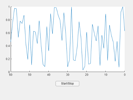
Plots in Apps: Improved responsiveness of axes interactions within apps
Responsiveness is improved for panning, rotating, and zooming into a region of
interest within a plot. To observe the improvement, the plot must be created in an app
or in a figure created with the uifigure function. The improvement is most noticeable for plots with
large numbers of points, or those that involve complex effects such as lighting,
transparency, or texture maps. Systems equipped with modern GPUs are more likely to show
the improvement.
For example, create a 3-D scatter plot with 200,000 points. If you run this code on a Windows 10, Intel Xeon CPU W-2133 @ 3.60 GHz test system with an NVIDIA Quadro® P620 GPU, and then drag to rotate the plot, the rotation is smoother and responds more quickly to the drag gesture than in the previous release.
z = linspace(0,4*pi,200000);
x = 2*cos(z) + rand(1,200000);
y = 2*sin(z) + rand(1,200000);
f = uifigure; a = axes(f);
scatter3(a,x,y,z,"filled")
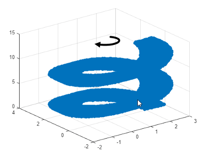
Plots in Apps: Improved responsiveness of axes interactions in plots with two y-axes
Responsiveness is improved for panning, rotating, and zooming into a region of
interest within a UIAxes or Axes object in MATLAB
Online that contains a chart created with yyaxis and a legend. For such charts, updates are faster, and
interactions are smoother in R2022a than in the previous release.
For example, create a UIAxes object with two
y-axes and a legend. If you run this code on a Windows 10, Intel
Xeon CPU E5-1650 v4 @ 3.60 GHz test system, when you drag the cursor to pan the
view of a UIAxes object, the axes pan faster and track the cursor more
closely in R2022a than in R2021b.
f = uifigure;
a = uiaxes(f);
plot(a,1:100,rand(1,100));
yyaxis(a,"right");
plot(a,1:100,linspace(1,10,100));
legend(a);
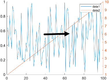
Plots in Apps: Faster animations in apps when multiple figures are open
Animations show improved performance in apps when multiple figures are open. To
observe the improvement, all figures must be created with the uifigure function.
For example, this code opens 10 empty figures and an additional figure containing a plot. The plot displays one marker that traces the path of a line at every iteration of a loop. The loop is about 6x faster than in the previous release.
function movingmarker % Open 10 empty figures for n = 1:10 uifigure("Position",[10+n*3 10+n*3 200 200]); end % Create a figure and a plot with one marker uif = uifigure; x = linspace(0,10,200); y = sin(x); ax = axes(uif); p = plot(ax,x,y,"-o","MarkerIndices",1); % Move the marker along the sine wave tic for idx = 2:200 p.MarkerIndices = idx; drawnow end toc end
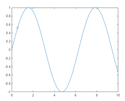
The approximate execution times for the loop are:
R2021b: 32.6 s
R2022a: 5.4 s
The code was timed on a Windows 10, Intel
Xeon CPU W-2133 @ 3.60 GHz test system by calling the
movingmarker function.
Property Inspector: Improved performance when opening for the first time
The Property Inspector for a figure window shows improved performance when opening for
the first time in a MATLAB session. The delay between clicking the Property Inspector icon or calling
inspect and the inspector being ready is reduced. The
improvement is most noticeable as the plot in the figure window becomes more
complex.
For example, open the Property Inspector for a plot of a 5-by-5 matrix by calling
inspect. If you run this code on a Windows 10, Intel
Xeon CPU E5-1650 v4 @ 3.60 GHz test system, you can use the Property Inspector
sooner in R2022a than in R2021b.
r = rand(5,5); p = plot(r); inspect(p)
Projects: Reduce test runtime in continuous integration workflows using the dependency cache
You can now specify where your project stores the dependency analysis results. In
agile development workflows that use Git™ and a continuous integration (CI) server, share the dependency cache file
(.graphml) to run an incremental dependency analysis and reduce
the test suite runtime. See Continuous Integration Using MATLAB Projects and Jenkins.
To set the project dependency cache file, on the Project tab, in the Environment section, click Details. In Dependency cache file, browse to and specify a GraphML file. If the cache file does not exist, the project creates it for you.
Alternatively, you can create and set the project dependency cache programmatically:
matlab.project.example.timesTable
proj = currentProject;
proj.DependencyCacheFile = "myProjectCacheFile"Dependency Analyzer: Save dependency graph as image
You can now save the dependency analysis results as an image. See Export Dependency Analysis Results.
Code Compatibility Analyzer App: Identify and address compatibility issues against current version of MATLAB
The MATLAB Code Compatibility Report is now available as an app. You can access the
Code Compatibility Analyzer from the apps gallery in MATLAB or from the command line using
codeCompatibilityAnalyzer. For more information, see MATLAB Code Compatibility Analyzer.
Unit Testing Framework: Create test classes interactively using the Current Folder browser
You can now create a test class using the Current Folder browser in MATLAB and MATLAB Online. To create a new test class, right-click in the Current Folder browser and then select New > Test Class.
Unit Testing Framework: Create temporary folders that are automatically removed
The matlab.unittest.TestCase class has a new method createTemporaryFolder that creates a temporary folder for your tests. The
lifecycle of the folder is tied to the test case. Once the test case goes out of scope,
the testing framework removes the folder.
Unit Testing Framework: Generate DOCX, HTML, and PDF reports after test execution
The matlab.unittest.TestResult class has three new methods that enable
you to generate various test reports from test results. You can run your tests and
collect the test results, and then generate test reports from part or all of your results:
To generate a DOCX report from the test results, use the generateDOCXReport method.
To generate an HTML report from the test results, use the generateHTMLReport method.
To generate a PDF report from the test results, use the generatePDFReport method.
With this feature, you are no longer required to run tests using a TestReportPlugin instance. For example, run your tests and then generate an
HTML report from the test results. Save the report as report.html in
a folder named myResults.
suite = testsuite("MyTestClass"); runner = testrunner; results = run(runner,suite); generateHTMLReport(results,"myResults",MainFile="report.html")
Unit Testing Framework: Debug uncaught errors in tests
Starting in R2022a, when a test runner with a StopOnFailuresPlugin instance encounters an uncaught error, MATLAB enters debug mode at the source of the error and lets you use debugging
commands to investigate the cause of the error. In previous releases, while the plugin
stops the test run to report the error, debugging capabilities are limited because the
error disrupts the stack.
Unit Testing Framework: Collect statement and function coverage metrics for your source code
Starting in R2022a, when you generate an HTML code coverage report using the CoverageReport format, the report displays statement and function coverage metrics:
Use statement coverage to see whether every MATLAB statement in your source code is executed at least once.
Use function coverage to see whether every function in your source code is called at least once.
In previous releases, you can generate only line coverage metrics for your source code. Compared to line coverage, statement and function coverage provide a more detailed analysis of the source code covered by the tests.
Functionality being removed or changed
pack function will be removed in a future release
Warns
The pack function will be removed in a
future release. There is no replacement for this function because you do not need to
use it on a 64-bit system. For more information about strategies for reducing memory
usage, see Strategies for Efficient Use of Memory and Resolve “Out of Memory” Errors.
matlab.unittest.TestSuite.fromFolder includes tests from package
folders when creating a test suite
Behavior change
Starting in R2022a, the matlab.unittest.TestSuite.fromFolder method treats folders and
packages the same way, and includes tests defined within package folders when
creating a test suite. For example, suite =
matlab.unittest.TestSuite.fromFolder(pwd,IncludingSubfolders=true)
creates a suite from all the test files in the current folder and any of its
subfolders, including package folders. In previous releases, the method ignores any
tests defined in a package folder and its subfolders.
This behavior change also applies to the testsuite, runtests, and runperf functions when they operate on a folder containing tests.
With the consistent treatment of folders and packages, creating a suite from all
test files within a folder and its subfolders becomes more convenient and
independent of the folder structure.
To exclude tests defined within packages, filter the suite being constructed or
returned by fromFolder. For example, create a filtered test suite
comprising tests whose names do not include any dots (that is, do not refer to any
packages).
import matlab.unittest.TestSuite import matlab.unittest.selectors.HasName import matlab.unittest.constraints.ContainsSubstring suite = TestSuite.fromFolder(pwd,HasName(~ContainsSubstring(".")), ... IncludingSubfolders=true);
builddocsearchdb creates searchable database with new
name
Behavior change
When building a searchable documentation database for custom toolboxes, the
builddocsearchdb function now creates
the subfolder helpsearch-v4 to contain the search database files.
Previously, builddocsearchdb created a subfolder named
helpsearch-v3.
To ensure the documentation for the custom toolbox is searchable in R2022a, run
builddocsearchdb against your help files using MATLAB R2022a. Maintain the helpsearch-v4 subfolder
containing the search database files created in R2022a and the
helpsearch-v3 subfolder containing the search database files
created in previous releases side by side. Then, when you run any MATLAB release, the Help browser automatically uses the appropriate database
for searching your documentation.
C++ Interface: Array size help text for functions and methods
If a function or method takes a clib or MATLAB array, the generated help text displays size information for the argument. For more information, see Array Size Help for Functions and Methods.
C Interface: Build third-party C library interface using
clibgen.generateLibraryDefinition
Create interfaces for libraries with C files that are built with C compilers using
clibgen.generateLibraryDefinition. Use this function to get the benefits
of publishing an interface as described in Build MATLAB Interface to C++ Library instead of
calling the loadlibrary function described in Call C from MATLAB.
For information about using clibgen.generateLibraryDefinition
with C files, see Files in Your
Library under the Tips section. To build
an interface to C libraries, use the CLinkage name-value argument.
C++ Interface: Support for C++ language features
The C++ interface supports these additional C++ language features.
std::complex support for complex scalars and arrays for
fundamental types of double, float,
int8, uint8, int16,
uint16, int32,
uint32, int64, and
uint64. For information about mapping these types to
MATLAB data, see Numeric Types.
If the size of a 1-D array parameter is not specified, you can represent the
size in MATLAB using multiple dimensions. For example, the input to this function is a
2-D array mat of size
len-by-typeSz.
void readMatrix2DArr(int const [] mat, size_t len, size_t typeSz)
You can specify the SHAPE of the argument as
["len","typeSz"]. For more information, see Define Missing SHAPE Parameter.
std::vector as data member.
C++ Interface: Publisher options
The C++ interface supports these build configuration features.
Specify compiler and linker flags used to build an interface. Use the
AdditionalCompilerFlags or AdditionalLinkerFlags name-value arguments in clibgen.generateLibraryDefinition or clibgen.buildInterface to pass flags to the compiler and linker.
These functions do not validate the flags. The publisher needs to know how the
flags affect the build process. For more information, see Build C++ Library Interface and Review Contents.
Build an interface using a specific compiler standard. For example, to build a library
defined by A.hpp with C++17, type:
clibgen.generateLibraryDefinition("A.hpp",AdditionalCompilerFlags="-std=c++17")
For more information, see Specify C++ Compiler Standard.
Include static libraries with .a file extension on
Linux® and macOS platforms, and on Windows if the library is compiled with a supported MinGW® compiler. To include a static library, use the Libraries name-value argument in clibgen.generateLibraryDefinition or clibgen.buildInterface.
Call MATLAB from C++: Generate C++ code Interface for MATLAB Packages, Classes, and Functions
The matlab.engine.typedinterface.generateCPP creates a C++ header file from
MATLAB packages, classes, and functions. For more information, see What is Strongly Typed Interface for C++?.
MATLAB Data Array API: matlab::data::Array support for
row-major order
The MATLAB data array API supports iterating through the data of a
matlab::data::Array in either row-major or column-major order.
For information about specifying the layout when creating an array, see the
inputLayout parameter for createArray. For information about
iterating through an array, see matlab::data::ColumnMajor, matlab::data::ColumnMajorIterator<T>, matlab::data::RowMajor, and matlab::data::RowMajorIterator<T>.
MEX Functions: UTF-8 system encoding on Windows platforms
MATLAB now uses UTF-8 as its system encoding on Windows, completing the adoption of Unicode across all supported platforms. System calls made from within a MEX file take and return UTF-8 encoded strings. If your MEX file contains code or links to third-party libraries that assume a different system encoding, then you might see garbled text and thus need to update the code to be Unicode compliant.
Python: Use Name=Value syntax to pass keyword arguments to
Python functions
Python: Convert Python
list and tuple types to MATLAB types
You can convert Python
list and tuple types using MATLAB string and numeric converters. For details, see the
py.list and py.tuple entry in the Explicitly Convert Python Types to MATLAB Types table. For
examples, see Use Python list Variables in MATLAB and Use Python tuple Variables in MATLAB.
Conversion functions might not work on lists or tuples that contain elements which cannot be converted to the requested type:
double(py.list({3.0, 'MATLAB'}))Error using py.list/double Conversion of Python element at position 2 to type 'double' failed. All Python elements must be convertible as scalar to the requested type. Related documentation
For the related documentation, see Error Converting Elements of list or tuple.
Perl 5.34.0: MATLAB support on Windows
As of R2022a, MATLAB on Windows ships with an updated version of Perl, version 5.34.0.
If you use the perl command on Windows platforms, see https://www.perl.org/ for
information about using this version of the Perl programming language.
Compilers: Support for Microsoft Visual Studio 2022
As of R2021b Update 3, MATLAB supports Microsoft Visual Studio® 2022 for building C and C++ interfaces, MEX files, and standalone MATLAB engine and MAT-file applications.
Functionality being removed or changed
Python: Version 3.7 is no longer supported
Errors
Support for Python version 3.7 is discontinued. For continued support for your applications, upgrade to a supported version of Python. For supported version information, see Versions of Python Compatible with MATLAB Products by Release.
MEX file macro FORTRAN_COMPLEX_FUNCTIONS_RETURN_VOID has been
removed
Behavior change
For MEX files built in R2021b and earlier, MATLAB provided a macro,
FORTRAN_COMPLEX_FUNCTIONS_RETURN_VOID, to handle
platform-dependent calling syntax differences for passing complex numbers to Fortran
BLAS and LAPACK functions. As of R2022a, you no longer need a different calling
syntax on different platforms, and the macro for handling this difference has been
removed.
To update your code, replace statements such as these using
FORTRAN_COMPLEX_FUNCTIONS_RETURN_VOID:
/* Call BLAS function */ /* Use a different call syntax on different platforms */ #ifdef FORTRAN_COMPLEX_FUNCTIONS_RETURN_VOID zdotu(&result, &nElements, zinA, &incx, zinB, &incy); #else result = zdotu(&nElements, zinA, &incx, zinB, &incy); #endif
with:
/* Call BLAS function */ zdotu(&result, &nElements, zinA, &incx, zinB, &incy);
See dotProductComplex.c.
NET.addAssembly no longer removes leading spaces for
Windows drive letter paths
Behavior change
Before R2022a, on Windows platforms, the NET.addAssembly function removed
leading spaces in paths specifying the drive letter. If the full path to your
assembly is invalid with leading spaces, then remove the spaces before calling
NET.addAssembly.