MATLAB Install: Reduce footprint using default installation without local documentation
Starting in R2023a, the documentation is not installed as part of a MATLAB® or other product installation. This change significantly reduces the installation footprint of products. In most cases, not installing the documentation has no effect on the availability of documentation, as the Help Center displays the web documentation by default.
The documentation is not installed as part of a product installation. If you run MATLAB on a system with no internet connection (permanently offline), or if you plan to work offline occasionally on an otherwise internet-connected machine, you can install the documentation on your computer after installing products. For more information, see Install Documentation.
Editor: Interactively increment numeric values within section and run section after every change
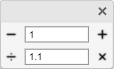
You can increment, decrement, multiply, or divide numeric values in the Editor and then run the current section after every change. This workflow can help you fine-tune and experiment with your code.
To adjust a numeric value, select the value or place your cursor next to the value. Next, right-click and select Increment Value and Run Section. In the dialog box that appears, specify a step value for addition and subtraction or a scale value for multiplication and division. Then, click one of the operator buttons to add to, subtract from, multiply, or divide the selected value in your section. MATLAB runs the section after every click.
Live Editor Controls: Add file browser to select file interactively in live script
You can add a file browser to your live script to interactively select a file by
opening a file selection dialog box. To add a file browser, go to the Live
Editor tab, and in the Code section, click
Control. Then, select File
Browser.
![]()
For more information, see Add Interactive Controls to a Live Script.
Live Editor Controls: Align controls within a section when code is hidden
The Live Editor automatically left-aligns drop-down lists, edit fields, numeric sliders, and numeric spinners within a block of code when the code is hidden.
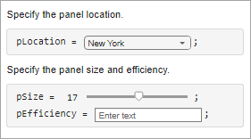
For example, this live script contains three controls in two different blocks of code. When the code is visible, the controls appear inline with the code.
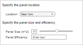
When the code is hidden, the Live Editor automatically aligns the second and third controls, as they are in the same block of code. The first control is not in the same block of code and is therefore not aligned to the other two controls.
The Live Editor does not align check boxes, buttons, and file browsers.
Desktop Layout in MATLAB Online: Access desktop tools and change the desktop layout using sidebars
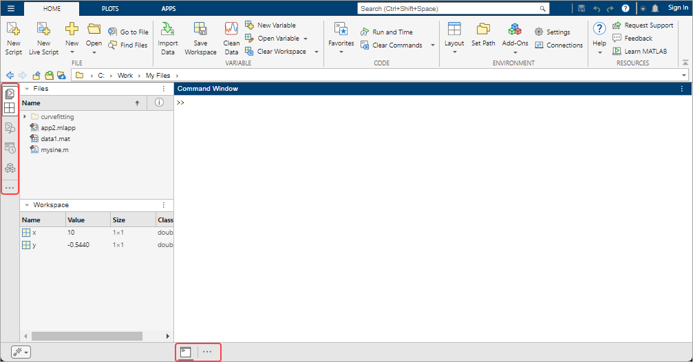
The MATLAB Online™ desktop includes sidebars on either side of the desktop to access desktop tools and change the desktop layout. The sidebars show the tools, such as the Workspace panel and the Files panel, that are docked on either side of the desktop. If there are no tools docked on one side, the sidebar for that side is hidden. You can use the sidebars to show and hide tools, group them together, and move them from one location to another.
When a tool is docked on the left or right side of the desktop, the sidebar on that side displays an icon for the tool. To show or hide the tool, click its icon in the sidebar. To show and hide multiple tools together, group them by dragging one of the tool icons next to another tool icon. To move a tool to a different location on the desktop, drag the tool or the icon for the tool to the new location. If there are no tools docked on one side, then the sidebar on that side is hidden.
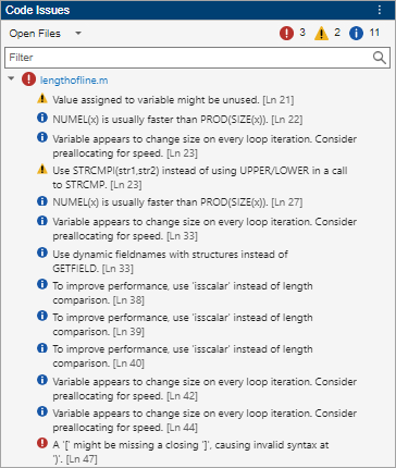
Code Issues Tool in MATLAB Online: Check code for errors and warnings using Code Issues tool
You can use the Code Issues tool to view error and warning messages about your code. The Code Issues tool displays the coding problems found by the MATLAB Code Analyzer as it automatically checks your code. Using the Code Issues tool, you can choose to view the errors and warnings for the current file or for all open files. You also can filter the list of messages by type (error or warning) as well as by message text.
To open the Code Issues tool, go to the Editor or Live
Editor tab, and in the Analyze section, click
Code Issues. By default, the Code Issues tool opens on the right
side of the desktop. To hide the Code Issues tool, click the Code Issues
icon in the sidebar.

Find Files Tool in MATLAB Online: Search for files with improved Find Files tool
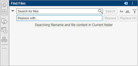
You can use the improved Find Files tool to search for files based on name or content.
When searching, you can choose whether to match the case of your search text as well as
whether to match the whole word. You also can select what folder to search in and filter
results by file extension. To search for files, click the Find Files icon
in the sidebar on the left side of the MATLAB
Online desktop.
Editor in MATLAB Online: Edit read-only files
You can now edit read-only files in MATLAB Online. When you save the file, MATLAB prompts you to overwrite the file or save the file using a different name.
Search in MATLAB Online: Access videos using Search box
In MATLAB Online, you can now use the Search box in the upper-right corner of the desktop to easily access videos that show you how to use MathWorks® products. In addition to videos, the Search box results include toolstrip actions, preferences, and Help Center resources such as functions, blocks, examples, and answers. To navigate to the Search box using a keyboard, press Ctrl+Shift+Space (or Command+Shift+Space on macOS systems).
loadenv Function: Load environment variables from
.env and plain text files
You can load environment variables from a .env or other plain text
file by using the loadenv
function. By using a .env file you can separate sensitive
configuration data from code and provide different sets of configurations for different
workflows.
Comparison Tool: Save text comparison results as PDF or DOCX reports programmatically and interactively
You can now use the Comparison Tool to programmatically and interactively publish text
comparison results as PDF or DOCX reports. For more details, see Compare Text Files and visdiff.
Toolbox Packaging: Specify packaging options when creating custom toolbox programmatically
When creating a custom toolbox programmatically using the matlab.addons.toolbox.packageToolbox function, you can specify packaging
options using a ToolboxOptions object. Using the
ToolboxOptions object, you can specify information about the toolbox
including what platforms the toolbox supports and what MATLAB releases the toolbox is compatible with. You also can specify what files
to package and what additional software to install with the toolbox. For an example, see
Specify packaging options using ToolboxOptions object.
Functionality being removed or changed
XML comparison type for visdiff function will be
removed
Still runs
The XML comparison type for the visdiff function will be removed in a future release. Overriding the
default comparison type by specifying "xml" will not be supported
in a future release. In R2023a, scripts that use
visdiff(filename1,filename2,"xml") continue to work.
lookfor function searches help text in third-party and
user-authored MATLAB program files
Behavior change
The lookfor function searches help text
in third-party and user-authored MATLAB program files. In R2022b, lookfor does not search
help text in third-party and user-authored MATLAB program files.
Code Analyzer: Enable custom checks and configure existing checks
You can configure existing checks displayed in the MATLAB editor by the Code Analyzer
and add custom checks by placing a file named
codeAnalyzerConfiguration.json in a resources folder. The
configuration file is effective in the folder containing the resources folder and any
subfolders.
You can modify existing Code Analyzer checks, including whether the check is enabled and its severity, message text, and parameters if the check has any, such as to limit the number of input and output arguments for a function. You can also create custom checks that trigger when specific functions are used. For more information on configuring Code Analyzer checks, see Configure Code Analyzer.
Validate your codeAnalyzerConfiguration.json configuration file for
proper formatting by using matlab.codeanalysis.validateConfiguration.
fix Function: Fix code issues from the command line
Fix certain code issues directly from the command line using the
fix function on codeIssues objects.
For example, create a script file with the following code:
x = [1 2 3] for n = 1:3 y(n) = x end
Run codeIssues on the file to identify code issues.
issues = codeIssues("exampleScript")issues =
codeIssues with properties:
Date: 03-Nov-2022 10:46:40
Release: "R2023a"
Files: "C:\MyCode\exampleScript.m"
CodeAnalyzerConfiguration: "active"
Issues: [3×10 table]
SuppressedIssues: [0×11 table]
Issues table preview
Location Severity Fixability Description CheckID LineStart LineEnd ColumnStart ColumnEnd FullFilename
_________________ ________ __________ ______________________________________________________________________________________________________________ _______ _________ _______ ___________ _________ ___________________________
"exampleScript.m" info auto "Add a semicolon after the statement to hide the output (in a script)." NOPTS 1 1 3 3 "C:\MyCode\exampleScript.m"
"exampleScript.m" info manual "Variable appears to change size on every loop iteration (within a script). Consider preallocating for speed." SAGROW 3 3 5 5 "C:\MyCode\exampleScript.m"
"exampleScript.m" info auto "Add a semicolon after the statement to hide the output (in a script)." NOPTS 3 3 10 10 "C:\MyCode\exampleScript.m"
Note that if the value for Fixability is auto
then the issue can be fixed using fix. Issues with
manual will not be fixed. Use fix to apply the
recommended fix to the issue identified.
fix(issues,"NOPTS")ans =
codeIssues with properties:
Date: 03-Nov-2022 10:47:04
Release: "R2023a"
Files: "C:\MyCode\exampleScript.m"
CodeAnalyzerConfiguration: "active"
Issues: [1×10 table]
SuppressedIssues: [0×11 table]
Issues table preview
Location Severity Fixability Description CheckID LineStart LineEnd ColumnStart ColumnEnd FullFilename
_________________ ________ __________ ______________________________________________________________________________________________________________ _______ _________ _______ ___________ _________ ___________________________
"exampleScript.m" info manual "Variable appears to change size on every loop iteration (within a script). Consider preallocating for speed." SAGROW 3 3 5 5 "C:\MyCode\exampleScript.m"
Code Analyzer App: Apply fixes to code issues interactively
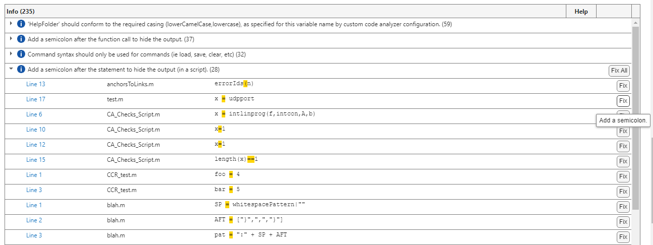
Fix certain code issues directly from the Code Analyzer app using the Fix button.
dictionary Object: Access and assign dictionary cell values with
curly braces
Data in cells can be looked up and assigned directly using curly
braces, {}. When dictionary values are cells,
a lookup using parentheses, (), returns a cell. Accessing the
contents of that cell requires indexing into the cell. This feature allows contents of
cell values to be accessed directly. For example, the dictionary d has three cell
values.
d =
dictionary (double ⟼ cell) with 3 entries:
1 ⟼ {["Hello"]}
2 ⟼ {[4 5 6]}
3 ⟼ {@sin} Perform a lookup using parentheses. The lookup returns the value as a cell containing an array.
d(2)
ans =
1×1 cell array
{[4 5 6]}Perform a lookup using curly braces. The lookup returns the value as an array.
d{2}ans =
[4 5 6]Output Argument Validation: Debug within output argument blocks
You can now use the MATLAB debugger within output arguments blocks of functions. While debugging an arguments block, the workspace is read-only. For more information on using the debugger, see Debug MATLAB Code Files.
Functionality being removed or changed
Warning about indexing with no subscripts
(MATLAB:subscripting:noSubscriptsSpecified) has been
removed
The warning about indexing into a built-in type with no subscripts
(MATLAB:subscripting:noSubscriptsSpecified) has been removed.
In previous releases, the warning was off by default, but when users opted in, the
warning would appear when indexing with no subscripts.
warning("on","MATLAB:subscripting:noSubscriptsSpecified"); x = [1 2 3 4 5]; y = x()
Warning: A value of class "double" was indexed with no subscripts
specified. Currently the result of this operation is the indexed value
itself, but in a future release, it will be an error.
y =
1 2 3 4 5Starting in R2023a, the behavior of indexing with no subscripts remains the same
and does not error, but the warning no longer appears. Using the
warning command to turn the warning on or off has no
effect.
Defining classes and packages: Using schema.m will not be
supported in a future release
Still runs
Support for classes and packages defined using schema.m files
will be removed in a future release. Replace existing schema-based classes with
classes defined using the classdef keyword.
pivot Function: Summarize tabular data using pivot table
Perform a pivoting operation on data in a table or timetable by using the pivot
function. Specify grouping variables that define variables or rows in the pivoted table
using colvars or rowvars.
Optionally define parameters such as the data variable, function to apply to the data variable, and grouping variable binning schemes by specifying name-value arguments.
table and timetable Data Types: Perform
calculations directly on tables and timetables without extracting their data
You can now perform calculations directly on tables and timetables without extracting their data. All the variables in your tables and timetables must have data types that support calculations. You can also perform operations where one operand is a table or timetable and the other is a numeric or logical array. Previously, all calculations required you to extract data from your tables and timetables by indexing into them.
For more information, see Direct Calculations on Tables and Timetables and Rules for Table and Timetable Mathematics.
Timetable Events: Find and label events in timetables using attached event tables
To find and label events in a timetable, attach an event table to it. An event table is a timetable of events. An event consists of an event time (when something happened), often an event length or event end time (how long it happened), often an event label (what happened), and sometimes additional information about the event. Event tables are designed to be attached to timetables. When you attach an event table to a timetable, you can find or label rows in the timetable that occur during events.
MATLAB provides these functions to create event tables from input data, filter timetable rows on event times, and synchronize events to timetables:
combinations Function: Generate all element combinations of
arrays
Generate all element combinations of arrays of varying sizes and data types by using
the combinations function. Each row of the output table is a combination.
Applying the combinations function is equivalent to finding the
Cartesian product of sets of elements.
fillmissing2 Function: Fill missing entries in two-dimensional
data
Fill missing entries in two-dimensional data sets using the fillmissing2 function. You can fill missing entries using interpolation
or moving window methods.
fillmissing Function: Use values from nearest neighbors to fill
missing data
You can use the 'knn' method of the fillmissing function to fill missing entries in your data with the
corresponding values in the nearest row, based on the pairwise Euclidean distance
between rows. You can optionally specify a value k for the
'knn' method to fill missing entries with the mean of the
corresponding values in the k nearest rows.
You can also specify a distance function, using the Distance
name-value argument, to measure the distance between rows with a specified metric.
Distance can have any of these values:
'euclidean' — Euclidean distance (default)
'seuclidean' — Scaled Euclidean distance
A function handle — User-specified distance function
Descriptive Statistics and Arithmetic: Omit or include missing data of multiple data types
When analyzing and preprocessing data, you can optionally specify to omit or include
numeric, datetime, duration, and categorical missing data. Use the
"omitmissing" or "includemissing" flags in
addition to any previously supported missing condition flags for these functions:
Find and Remove Trends Live Editor Task: Interactively find and remove periodic and polynomial trends
The Find and Remove
Trends task in the Live Editor can now identify periodic trends for
regularly spaced input data. Select the Periodic trend type, and
choose the SSA or STL
algorithm.
The task can also return polynomial and periodic trends, in addition to the detrended
data. Specify Output as Trends.
Previously, this task identified only polynomial trends and returned only the detrended data.
To reflect the enhanced functionality of finding and removing periodic and polynomial trends, this task in the Live Editor is now named Find and Remove Trends. Previously, this task was named Remove Trends.
Data Cleaner App: Save session as MAT-file and reload session
When working in the Data Cleaner app, save the session as a binary MAT-file containing the data and cleaning steps. To save the session file, in the File section of the Home tab, click Save. To reload the session, in the File section of the Home tab, click Open.
head and tail Functions: Get top or bottom
rows of array
groupsummary Function: Compute number of unique elements
Compute the number of distinct nonmissing elements in each group of data. Specify the
"numunique" or "all" method of the groupsummary function, or select the Number of unique
values or Select all computation method in
the Compute by
Group task in the Live Editor.
The "all" computation method now returns the number of unique
values in addition to the computation methods in the previous release.
movevars Function: Move table variables after last variable
without After name-value argument
When using the movevars
function, you can now move variables after the last variable without specifying the
After name-value argument.
For example, create a table. Then move the first variable after the last variable.
T = table([1;3;5],[2;4;6],[3;6;9])
T =
3×3 table
Var1 Var2 Var3
____ ____ ____
1 2 3
3 4 6
5 6 9
T = movevars(T,"Var1")
T =
3×3 table
Var2 Var3 Var1
____ ____ ____
2 3 1
4 6 3
6 9 5 In previous releases, calling movevars without specifying
either the After or Before name-value argument
resulted in an error. Moving a variable after the last variable required one of
these two syntaxes.
T = movevars(T,"Var1","After",width(T)) % or T = movevars(T,"Var1","After","Var3")
day Function: Return ISO day of week
To return the ISO day of week number, use the "iso-dayofweek"
option with the day function. In the ISO 8601 standard,
Monday is day 1 of the week.
For example, return the ISO day of week number for today.
D = datetime("today"); dayNumber = day(D,"iso-dayofweek")
week Function: Return ISO week of year or week of month
To return the ISO week of year number, use the "iso-weekofyear"
option with the week function. In the ISO 8601
standard, a week begins on Monday. Week 1 of a year is defined as the first week in the
year with at least four days.
To return the week of month number, use the "iso-weekofmonth"
option with the week function. A week begins on Monday. Week 1 of a
month is defined as the first week in the month with at least four days. ISO 8601 does
not specifically define the week of month number. However, this option returns a week of
month number that is consistent with the ISO week of year number.
For example, return the ISO week of year and week of month numbers for today.
D = datetime("today"); weekOfYear = week(D,"iso-weekofyear") weekOfMonth = week(D,"iso-weekofmonth")
Variables Editor: Edit categories of categorical table variable in MATLAB Online
In the MATLAB Online Variables editor, you can create, remove, or merge categories in a categorical table or timetable variable. To edit the categories, pause on the header of a categorical variable and click the triangle icon, or right-click the variable, and select Edit Categories.
Import Data Live Editor Task: Import data in live scripts
The Import Data Live Editor task allows you to import various types of data in a live script within a single framework. You can import these types of data:
MAT-file (for example, .mat)
Text (for example, .csv)
Spreadsheet (for example, .xlsx)
Image (for example, .png)
Audio (for example, .wav)
Video (for example, .avi)
To add the task to a live script in the Live Editor, click Task on the Live Editor tab and select the Import Data icon.
audiowrite Function: Write MP3 audio files
You can write MP3 audio files using the audiowrite function.
imfinfo Function: Get information about XMP metadata embedded in
JPEG files
The imfinfo function returns Extensible
Metadata Platform (XMP) metadata embedded in JPEG files in the
'XMPData' field of the output structure. The function also
returns International Press Telecommunications Council (IPTC) metadata embedded in the
XMP namespace. The IPTC data is stored in the 'Iptc4xmpCore' (core
metadata) and 'Iptc4xmpExt' (extension metadata) subfields of
'XMPData'.
Parallel Processing: Use readtable in thread-based
environments
You can use the readtable function in thread-based
environments. Parallel processing results in improved performance when reading data,
especially with remote data.
Scientific File Format Libraries: CDF library upgraded to version 3.8.1
The CDF library is upgraded to version 3.8.1.
Scientific File Format Libraries: CFITSIO library upgraded to version 4.1.0
The CFITSIO library is upgraded to version 4.1.0.
Functionality being removed or changed
web function will return handle to most recent MATLAB web browser as MATLAB class
Behavior change in future release
In a future release, the web function will return a handle to the most recent MATLAB web browser as a MATLAB class. Currently, the web function returns the
handle as a Java® class. With this change, some methods that were previously supported
in the returned handle will no longer be supported.
In most cases, you will not need to make any changes to your code. However, if you are using methods that are not supported in the returned MATLAB class, you will need to update your code.
MATLAB Support Package for Quantum Computing: Build, simulate, and run quantum algorithms
The MATLAB Support Package for Quantum Computing enables you to:
Build circuits to implement quantum algorithms using a variety of built-in gate functions.
For a complete list of built-in gate functions, see Types of Quantum Gates.
Leverage composite gates to create custom gates from available built-in gates, capture complex operations, and organize circuits.
Verify implementation of quantum algorithms with simulations on your local computer. Analyze simulation results to determine the outcome of a measurement.
Run gate-based quantum algorithms by connecting to quantum hardware on Amazon® Web Services (AWS®).
See Quantum Computing and Introduction to Quantum Computing for more information.
To install the MATLAB Support Package for Quantum Computing, locate the support package in Add-On Explorer using the instructions in Get and Manage Add-Ons.
pageeig Function: Perform eigenvalue decomposition on pages of
N-D arrays
Use the pageeig
function to calculate eigenvalues and eigenvectors of the pages of N-D arrays. In this
context, the N-D array is treated as a container for several 2-D matrices.
randi Function: Create random logical array
Use randi to create a random logical array by
specifying the typename argument as "logical" or
the prototype p as a logical array.
For example, you can create a 5-by-5 random logical array using randi([0
1],5,"logical").
Functionality being removed or changed
spy plots have adjusted default behavior for aspect ratio
and marker size
Behavior change
The aspect ratio of spy plots has a 1-to-10 limit,
after which the plot stops adjusting to the matrix shape. You can use
pbaspect("auto") for no special aspect ratio or
pbaspect([size(A,2) size(A,1) 1]) for the previous behavior
of a matching aspect ratio, even for very "squeezed" cases.
Additionally, the default marker size is based only on the matrix size. Previously, the point size of the axes on creation could also affect the marker size.
sky Function: Apply monochromatic colormap to charts
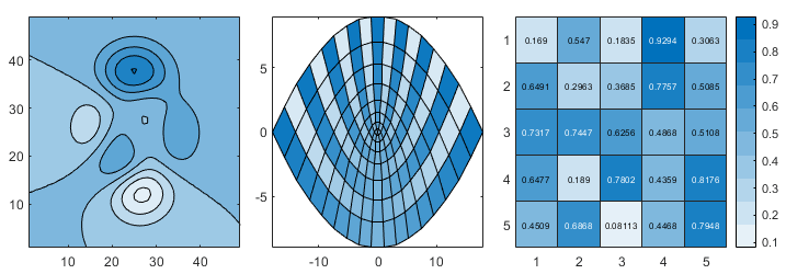
Use the sky
function to color charts with the same monochromatic colormap that heatmap charts use.
Like for all predefined colormaps, you can optionally specify the number of colors for
the sky colormap.
tiledlayout Function: Create horizontal or vertical
layouts
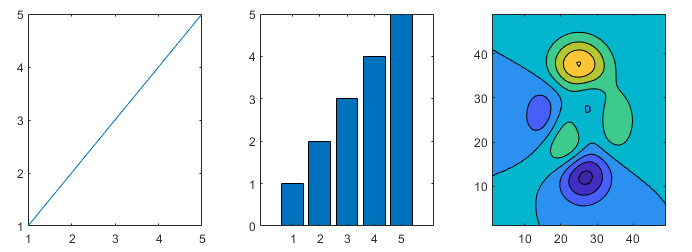
Create horizontal or vertical layouts by specifying "horizontal" or
"vertical" as the first input argument to the tiledlayout function. For example, create a horizontal layout and add
three plots.
tiledlayout("horizontal")
x = 1:5;
nexttile
plot(x)
nexttile
bar(x);
nexttile
contourf(peaks)
animatedline Function: Create animated lines using numeric,
datetime, or duration data
Use the animatedline function to create
animated lines using single, double, integer, datetime, or duration data for the
x-, y-, and
z-coordinates.
Grid Lines: Customize grid line thickness
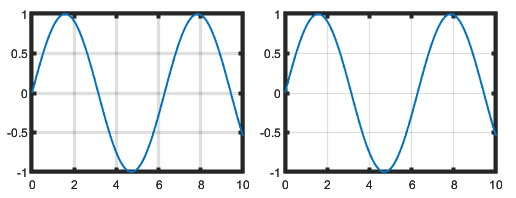
Change the thickness of grid lines independently of the box outline and tick marks by
setting the GridLineWidth and MinorGridLineWidth properties of the axes. Before R2023a, the
LineWidth property of the axes was the only property for
controlling the grid line width. However, that property controlled the grid lines, box
outline, and tick marks together. Now you can control the thickness of the grid lines
separately.
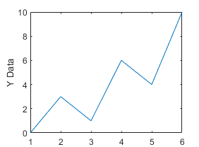
Axes Labels: Rotate x- and y-axes labels without overlapping the axes
When you change the Rotation property of
an axis label in a 2-D plot, the HorizontalAlignment and
VerticalAlignment properties of the label automatically change
to prevent overlap between the label and the axes.
For example, create a plot with a y-axis label.
plot([0 3 1 6 4 10])
ylab = ylabel("Y Data");
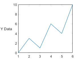
Rotate the label so that the text is horizontal. MATLAB automatically adjusts the HorizontalAlignment and
VerticalAlignment properties to prevent the overlap.
ylab.Rotation = 0;
Plotting Series of Lines: Control cycling order of line styles
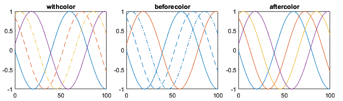
When plotting a series of multiple lines, you can use the LineStyleCyclingMethod property of the axes to control how different
lines are distinguished from one another. Specify this property as one of these values:
"withcolor" — Cycle through the line styles with the
colors
"beforecolor" — Cycle through the line styles before
cycling through the colors
"aftercolor" — Cycle through the line styles after
cycling through the colors (default)
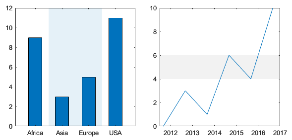
Plotting Series of Lines: Control whether the data range of a line affects automatic axes limits
Specify whether a specific line affects the automatically selected axes limits by
setting the AffectAutoLimits property. By default, the axes limits change to
encompass the data range for each successive line you create. Setting this property
enables you to focus on the range of a subset of lines in the axes.
![Two line plots, each showing the same two data sets as a thin red line and thick blue line, but with different x-axis limits. The x-values of the thin red line range from –100 to 100. The x-values of the thick blue line range from 0 to 100. The x-axis in the left plot spans the range [–100, 100]. The x-axis in the right plot spans the range [0, 100]. As a result, the right plot excludes part of the thin red line.](23a-graphics-affectsaoutolims-for-gr.png)
DatetimeRuler Object: Set or get the reference date for plotting
datetime values
Set the ReferenceDate property of a DatetimeRuler object when
you plot datetime values. This property is useful for synchronizing tick placement
across different axes and for plotting data from different time zones together.
Image Display Preferences: Access and update imshow preferences
in MATLAB
Online
In MATLAB
Online, you can set the default values for these aspects of images displayed
using imshow:
Axes visible — Control whether
imshow displays images with the axes box outline
and tick labels.
Border Style — Control whether
imshow draws a tight or loose border around images
in the figure window.
Initial Magnification — Control whether
imshow initially fits images to the figure window
or magnifies them by a specified percentage.
To open these image display preferences, on the Home
tab, in the Environment section, click
Preferences. Select MATLAB > Image Display.
Functionality being removed or changed
BaseValue property of bar,
stem, and area plots no longer changes
with axes limits
Behavior change
The BaseValue property of bar, stem, and area plots no longer depends on the axes limits. The property value
stays the same when you change axes limits or pan within the axes.
This change does not affect the appearance of the plots, but it provides a more predictable experience when you change the axes limits or pan within the axes.
MATLAB
Online limits imshow image display resolution
Behavior change
MATLAB
Online limits the maximum imshow image display resolution to
improve rendering speeds for large images. This behavior affects the on-screen
display, but it does not affect the image data. Before displaying an image,
imshow resizes the largest dimension to a maximum size of
512 pixels. The smaller dimension adjusts to preserve the aspect ratio of the image.
To view images at their full resolution, use MATLAB desktop or set the MaxRenderedResolution property
of the output Image object to "none". For
details about the MaxRenderedResolution property, see Image Properties.
Plot Catalog tool will be removed
Warns
The Plot Catalog tool will be removed in a future release. Instead, to interactively create and explore visualizations for your data, use the Plots tab in the MATLAB Toolstrip or the Create Plot task in the Live Editor.
For more information about visualizations, see Types of MATLAB Plots or toolbox-specific documentation.
Figure Tools menu will no longer include interaction modes and options
Still runs
In a figure, the Tools menu will no longer contain these items in a future release:
Zoom In
Zoom Out
Pan
Rotate 3D
Data Tips
Brush
Restore View
Options
Align Distribute Tool
Instead, to enable interaction modes, use the axes toolbar. Customize the
interaction by right-clicking in the chart when an interaction mode is enabled, or
for apps, by using the InteractionOptions property of the axes.
addStyle Function: Add styles to items in list box or drop-down UI
component
Create styles for specific items in a list box or drop-down UI component using the
uistyle
and addStyle
functions. For example, you can add icons to items in a list box. To get information on
applied styles, query the StyleConfigurations property of the
ListBox or DropDown object. To remove a style
from a component, use the removeStyle function.
uistack Function: Change stacking order of UI components in UI
figure
You can now use the uistack function to change the
stacking order of UI components and containers in a figure created using the
uifigure function. Previously, uistack
supported UI components only in figures created using the figure
function.
uipanel and uibuttongroup Functions: Specify
container border color
You can specify the border color of panels and button groups by using the
BorderColor property. For more information, see Panel Properties
or ButtonGroup Properties.
uihtml Function: Send events between MATLAB and HTML
When you create an HTML UI component using the uihtml
function, you can send events between MATLAB and HTML. Send events when a specific action occurs to one object and
another object needs to know about or react to that action. For example, you can send an
event from HTML to MATLAB whenever a user clicks a button HTML element, and then write a
callback in MATLAB that updates your app in response. You also can send an event from
MATLAB to HTML whenever a user clicks a Button UI component in
your app, and then write a callback in your HTML source file that updates the HTML code
in response.
To send an event from HTML to MATLAB, call the sendEventToMATLAB function on the
htmlComponent
JavaScript® object in your setup method.
htmlComponent.sendEventToMATLAB(eventName,eventData)
React to this event by writing MATLAB code that creates an HTMLEventReceivedFcn callback for
the HTML
MATLAB object.
comp.HTMLEventReceivedFcn = @myCallbackFunction
To send an event from MATLAB to HTML, call the sendEventToHTMLSource function on the
HTML
MATLAB object.
sendEventToHTMLSource(comp,eventName,eventData)
React to this event by writing JavaScript code in your setup method that listens for the event
and executes a callback function in response.
htmlComponent.addEventListener(eventName,eventData,callbackFunction)
For more information, see Send Event from JavaScript to MATLAB and Send Event from MATLAB to JavaScript.
uiimage Function: Specify image alt text for use with screen
readers
Provide a description of an image created using the uiimage
function by specifying the AltText property. This property is used by
screen readers to describe the image when an app user navigates through the app.
appmigration.migrateGUIDEApp Function: Programmatically migrate
existing GUIDE apps to App Designer
Programmatically migrate existing GUIDE apps to App Designer apps by using the
appmigration.migrateGUIDEApp function. You can specify a single app,
multiple apps, or a folder of apps to migrate as a batch. The function uses the
GUIDE to App Designer Migration Tool for MATLAB to perform the migration.
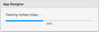
App Designer: View progress when loading an app
When you load an app in App Designer, a progress bar now displays an estimate of its loading progress.
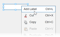
App Designer: Add label to unlabeled UI component
To add a label to a UI component without one, in Design View, right-click the component and select Add Label or use the keyboard shortcut Ctrl+L.
App Designer: Replace assigned callback with new callback
You can now more efficiently create a new callback for a UI component that already has
a callback assigned. To replace an existing callback with a new one, select the
component in the Component Browser and, in the
Callbacks tab, select the option to add a callback. For
example, for a component with a ButtonPushedFcn callback already
assigned, select <add ButtonPushedFcn callback> from the
associated drop-down list. App Designer creates a new callback function, assigns it to
the component, and unassigns the previous callback function.
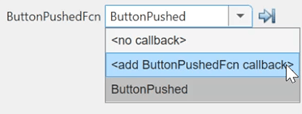
Previously, you had to first unassign the assigned callback from the component before creating a new callback.
App Testing Framework: Test context menus within labels
You can use the chooseContextMenu method to test a right-click that opens a context menu
within label components. For example, assign a context menu with two items to a label,
and then choose the first menu item.
fig = uifigure; lbl = uilabel(fig); cm = uicontextmenu(fig); m1 = uimenu(cm,Text="Menu1"); m2 = uimenu(cm,Text="Menu2"); lbl.ContextMenu = cm; testCase = matlab.uitest.TestCase.forInteractiveUse; testCase.chooseContextMenu(lbl,m1)
Axes Interactions: Customize behavior of interactions with axes view
For apps created in App Designer and using the uifigure function,
customize axes interaction behavior using the InteractionOptions
property of the axes. Customize the behavior of panning, zooming, rotating, adding data
tips, data brushing, and restoring the original view by setting the value of
InteractionOptions properties. For a complete list of properties,
see InteractionOptions
Properties.
The options set by the InteractionOptions object apply to these
interactions on the associated axes:
The built-in interactions specified by the
Interactions property of the axes
Interactions enabled by using mode functions, such as
pan and zoom
Interactions enabled using the axes toolbar
For example, limit all pan and zoom interactions to the x-dimension only.
fig = uifigure;
ax = uiaxes(fig);
ax.InteractionOptions.LimitsDimensions = "x";Plots in Apps: Enable data cursor mode
For apps created in App Designer and using the uifigure function,
use data cursor mode to interactively create and edit data tips. For supported charts,
select the Data Tips
icon in the axes toolbar or use the datacursormode function.
Plots in Apps: Specify axes for interaction mode
For apps created in App Designer and using the uifigure function,
set the interaction mode for axes. Specify the Axes object as the first
argument for these functions:
For example, for a figure with two axes, enable pan mode for only axes
ax1.
fig = uifigure;
t = tiledlayout(fig,1,2);
ax1 = nexttile(t);
ax2 = nexttile(t);
pan(ax1,"on")When setting the interaction mode for axes, these functions do not return
pan, zoom, rotate3d,
DataCursorManager, or brush objects. Previously,
these functions set the interaction mode for all Axes children of the
current or target figure.
Functionality being removed or changed
uistack function has different stacking behavior for menus,
toolbars, push tools, and toggle tools
Behavior change
When you modify the stacking order of menus, toolbars, push tools, and toggle
tools using the uistack function, the behavior is
different than in previous releases. For example, starting in R2023a, calling
uistack(comp,"up") has this behavior:
Menu items parented to a figure — The menu item moves one place to the left in the menu bar. Previously, the menu item moved one place to the right.
Menu items parented to a context menu — The menu item moves one place up in the context menu. Previously, the menu item moved one place down.
Toolbars — The toolbar moves one place up within the collection of toolbars in the figure. Previously, the toolbar moved one place down.
Push tools and toggle tools — The push tool or toggle tool moves one place to the left in the toolbar. Previously, the push tool or toggle tool moved one place to the right.
If your code uses uistack to modify the stacking order of
menus, toolbars, push tools, or toggle tools, make these updates to the code to
retain the previous behavior.
| Original Code in R2022b or Earlier | Updated Code in R2023a |
|---|---|
uistack(comp,"top") | uistack(comp,"bottom") |
uistack(comp,"up",step) | uistack(comp,"down",step) |
uistack(comp,"bottom") | uistack(comp,"top") |
uistack(comp,"down",step) | uistack(comp,"up",step) |
HighlightColor property of panel and button group containers
is not recommended
Still runs
Using the HighlightColor property to specify the border color
of a panel or button group is not recommended. Use the
BorderColor property instead. The
BorderColor property has the same effect and accepts the same
values as the HighlightColor property. For more information, see
Panel Properties or ButtonGroup Properties.
There are no plans to remove support for the HighlightColor
property at this time. However, the HighlightColor property no
longer appears in the list returned by calling the get function
on a UI container.
Language and Programming: Improved performance when calling functions and methods
Calling most functions and methods shows improved performance. For example, in a file
named myFun.m in your current folder, create the
myFun function.
function y = myFun(x) y = x; end
In a file named timingTest.m in your current folder, create a
function that calls myFun. The timingTest
function is about 1.6x faster than in the previous release.
function out = timingTest n = 1e7; for i = 1:n out = myFun(3); end end
The approximate execution times are:
R2022b: 0.18 s
R2023a: 0.11 s
The code was timed on a Windows® 10, Intel®
Xeon® CPU E5-1650 v4 @ 3.60 GHz test system using the
timeit function.
timeit(@timingTest)
Function Handles: Improved performance when invoking handles to named functions
Invoking handles to named functions that are not nested shows improved performance.
Invoking such function handles no longer results in an overhead compared to calling
functions directly. For example, in a file named myFun.m in your
current folder, create the myFun function.
function y = myFun(x) y = x; end
In a file named timingTest.m in your current folder, create a
function that invokes a handle to myFun. The
timingTest function is about 40x faster than in the previous
release.
function t = timingTest f = @myFun; n = 1e7; tic for i = 1:n out = f(3); end t = toc; end
The approximate execution times are:
R2022b: 4.4 s
R2023a: 0.11 s
The code was timed on a Windows 10, Intel
Xeon CPU E5-1650 v4 @ 3.60 GHz test system by calling the
timingTest function.
varargin Argument: Improved performance when specifying zero or
more inputs
Specifying a variable number of input arguments using varargin shows improved performance. For example, in a file named
timingTest.m in your current folder, create a function that
expects one input and accepts an additional number of inputs.
function timingTest(x,varargin) n = 1e6; tic for i = 1:n y = myFun(x,varargin{:}); end toc end function y = myFun(x,varargin) if nargin == 1 y = x; elseif nargin == 3 y = x + varargin{1} + varargin{2}; else y = NaN; end end
The amount of improvement depends on whether varargin is empty.
The performance improvement is most significant when varargin is
empty.
Empty varargin — Time this code by running
timingTest(1). The code is about 22x faster than in the
previous release. The approximate execution times are:
R2022b: 0.404 s
R2023a: 0.018 s
Nonempty varargin — Time this code by running
timingTest(1,2,3). The code is about 2x faster than in
the previous release. The approximate execution times are:
R2022b: 1.428 s
R2023a: 0.734 s
The code was timed on a Windows 10, Intel Xeon CPU E5-1650 v4 @ 3.60 GHz test system.
timetable Data Type Indexing: Improved performance when
subscripting with times or with withtol subscript
timetable subscripting when subscripting with times or with a
withtol subscript is significantly faster in R2023a than in
R2022b.
For example, when you use a vector of 100 datetime values
to subscript into a timetable that has 107 rows,
performance in R2023a is about 114x faster than in R2022b.
function timingTest() rng default % 10^7 rows N = 10000000; rowtimes = datetime(2023,1,1,0,0,0:N-1); rowtimes.Format = rowtimes.Format + ".SSS"; tt = timetable(rand(N,1),RowTimes=rowtimes); % 100 values chosen in steps of 10 n = 1000; t = datetime(2023,1,1,0,0,0:10:n-1); tic tt2 = tt(t,:); toc end
The approximate execution times are:
R2022b: 9.10 s
R2023a: 0.08 s
Similarly, when you use a vector of 100 duration values to
subscript into a timetable that has 107 rows,
performance in R2023a is about 14x faster than in R2022b.
function timingTest() rng default % 10^7 rows N = 10000000; rowtimes = seconds(0:N-1); tt = timetable(rand(N,1),RowTimes=rowtimes); % 100 values chosen in steps of 10 n = 1000; t = seconds(0:10:n-1); tic tt2 = tt(t,:); toc end
The approximate execution times are:
R2022b: 1.29 s
R2023a: 0.09 s
When you use a withtol subscript with a timetable that has
107 rows, performance in R2023a is about 44x
faster than in R2022b.
function timingTest() rng default % 10^7 rows N = 10000000; rowtimes = seconds(0:N-1); tt = timetable(rand(N,1),RowTimes=rowtimes); % 100 values chosen in steps of 10 n = 1000; t = seconds(0:10:n-1); tt.Time = tt.Time + .1*seconds(rand(N,1)); wt = withtol(t,seconds(.1)); tic tt2 = tt(wt,:); toc end
The approximate execution times are:
R2022b: 3.92 s
R2023a: 0.09 s
The code was timed on a Windows 10, AMD® EPYC 74F3 24-Core Processor @ 3.19 GHz test system by calling each version
of the timingTest function.
Complex Matrices: Improved performance when using colon indexing to copy complex matrices
Copying a complex matrix using colon indexing shows improved performance. This improvement is greater for larger matrices.
For example, this code is about 105x faster than in the previous release.
a = rand(100)*1j; tic; for i = 1:1e6 b = a(:,:); end toc;
The approximate execution times are:
R2022b: 22.3 s
R2023a: 0.212 s
This improvement is most noticeable when the copy is not modified. However, examples like these still execute noticeably faster.
Modify no elements of the copy based on a conditional (95x improvement).
a = rand(100)*1j; tic; for k = 1:1e6 b = a(:,:); if (isreal(b(1,1))) b(1,1) = b(1,1)*1j; end toc;
R2022b: 21.3 s
R2023a: 0.223 s
Modify an element of the copy based on a conditional (2x improvement).
a = rand(100)*1j; tic; for k = 1:1e6 b = a(:,:); if (~isreal(b(1,1))) b(1,1) = b(1,1)*1j; end toc;
R2022b: 23.5 s
R2023a: 10.1 s
Use an implicit copy in an operation (4x improvement).
a = rand(100)*1j; b = rand(100)*1j; tic; for k = 1:1e6 c = a(:,:) + b; end toc;
R2022b: 41.1 s
R2023a: 9.87 s
Resize from 4-D to 2-D during copy (63x improvement).
a = rand(10,10,10,10)*1j; tic; for k = 1:1e6 b = a(:,:); end toc;
R2022b: 28.2 s
R2023a: 0.451 s
The code was timed on a Windows 10, Intel Xeon CPU E5-2650 v2 @ 2.60 GHz test system.
mean, std, var, and
rmse Functions: Improved performance when computing along
default vector dimension
The mean, std, var, and rmse
functions show improved performance when computing over a real vector when the operating
dimension is not specified. The functions determine the default operating dimension more
quickly in R2023a than in R2022b.
For example, this code computes the mean along the default vector dimension. The code is about 2.2x faster than in the previous release.
function timingMean A = rand(10,1); for i = 1:8e5 mean(A); end end
The approximate execution times are:
R2022b: 0.91 s
R2023a: 0.41 s
The code was timed on a Windows 10, Intel
Xeon CPU E5-1650 v4 @ 3.60 GHz test system using the
timeit function.
timeit(@timingMean)
Moving Statistics Functions: Improved performance when computing over matrix with sample points
Moving statistics functions show improved performance when computing over a matrix when there are sample points. These functions show improved performance:
For example, this code computes the moving sums of a 300-by-300 matrix with corresponding sample points. The code is about 3x faster than in the previous release.
function timingMovsum A = randn(300); t = sort(rand(300,1)); tic for k = 1:2000 movsum(A,0.1,"SamplePoints",t); end toc end
The approximate execution times are:
R2022b: 1.04 s
R2023a: 0.34 s
The code was timed on a Windows 10, Intel
Xeon CPU E5-1650 v4 @ 3.60 GHz test system by calling the
timingMovsum function.
histcounts Function: Improved performance with small numeric and
logical input data
The histcounts function shows improved
performance for numeric and logical data due to faster input parsing. The performance
improvement is more significant when input parsing is a greater portion of the
computation time. This situation occurs when the size of the data to distribute among
bins is smaller than 2000 elements.
For example, this code calculates histogram bin counts for a 1000-element vector. The code is about 3x faster than in the previous release.
function timingHistcounts X = rand(1,1000); for k = 1:3e3 histcounts(X,"BinMethod","auto"); end end
The approximate execution times are:
R2022b: 0.62 s
R2023a: 0.21 s
The code was timed on a Windows 10, Intel
Xeon CPU E5-1650 v4 @ 3.60 GHz test system using the
timeit function.
timeit(@timingHistcounts)
fzero function: Improved performance
The fzero function shows improved
performance. The performance improvement is most significant when the objective function
is fast to compute and fzero does not use an options argument.
For example, this code runs about 4x faster than in the previous release.
rng default N = 1e5; levels = 1.5 * rand(N,1); out = zeros(N,1); myfun = @(x,lv)x*sin(x)-lv; tic for i=1:N out(i) = fzero(@(x)myfun(x,levels(i)),0); end toc
The approximate execution times are:
R2022b: 2.67 s
R2023a: 0.63 s
The code was timed on a Windows 10, Intel Xeon CPU E5-1650 v3 @ 3.5 GHz test system.
Plots in Apps: Improved performance when rerendering axes
Axes rerender more quickly in R2023a than in R2022b. The reduced rerendering time is most noticeable when many sequential updates to the axes occur.
For example, first create axes to specify as the input to the
timingAnimation function. Then, call the
timingAnimation function to add points to an animated line. The
time for the axes to rerender is reduced, resulting in an animation that is about 1.35x
faster in R2023a than in the previous
release.
function timingAnimation(ax) h = animatedline(ax); x = linspace(0,4*pi,1000); y = sin(x); tic for k = 1:length(x) addpoints(h,x(k),y(k)); drawnow end toc end
The approximate durations of the animation are:
R2022b: 5.66 s
R2023a: 4.20 s
The code was timed on a Windows 10, Intel
Xeon CPU E5-1650 v4 @ 3.60 GHz test system by calling the
timingAnimation function.
Plots in Apps: Improved performance when creating axes
Axes render more quickly within apps and within figures created with the
uifigure function in R2023a than in R2022b. The delay before
the axes appear in an existing figure is reduced.
For example, if you run the code uiaxes(f) for an existing figure
f, the axes appear about 3.7x faster in R2023a than in R2022b
when creating axes for the first time in a MATLAB session and about 2.4x faster for
subsequent axes.
The approximate axes rendering times are:
| First Axes | Subsequent Axes | |
|---|---|---|
| R2022b | 14.94 s | 1.06 s |
| R2023a | 4.02 s | 0.44 s |
These operations were timed on a Windows 10, Intel Xeon CPU E5-1650 v4 @ 3.60 GHz test system.
Plots in Apps: Improved responsiveness of ruler-pan interaction
The ruler-pan interaction is faster and smoother within apps and within figures
created with the uifigure function in R2023a than in R2022b. The
improvement is most noticeable for plots that display a large number of data
points.
For example, this code creates a figure with a plot of a 2500-by-2500 matrix. When you pan the ruler, the ruler-pan interaction is smoother and the axes track your mouse motion more closely in R2023a than in the previous release.
f = uifigure; ax = uiaxes(f); p = peaks(2500); plot(ax,p)
| R2022b | R2023a |
|---|---|
When panning the ruler, the surface plot takes a moment to reposition and jumps to the new location.
| When panning the ruler, the surface plot follows the mouse motion more closely and repositions more quickly at the new location.
|
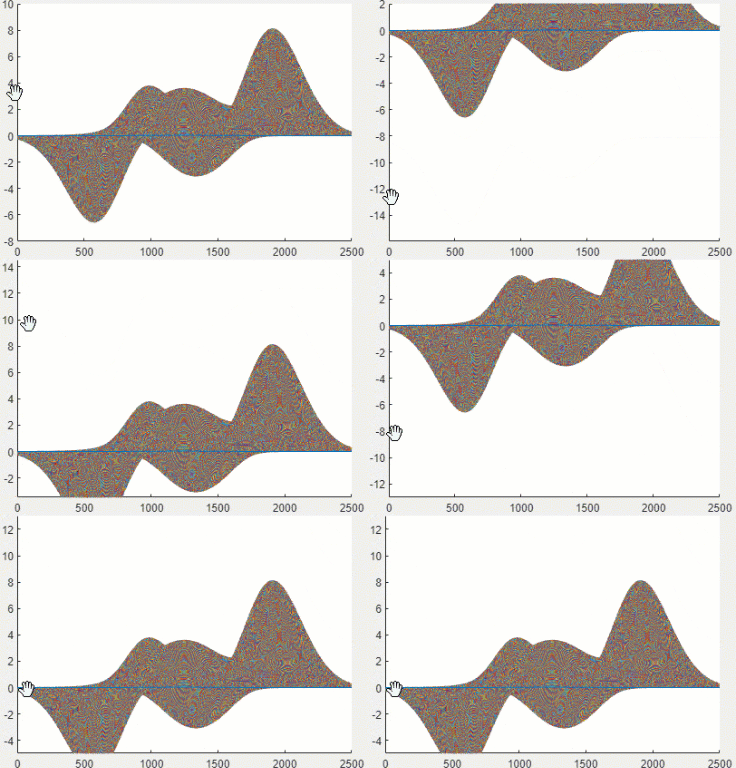
The ruler-pan interaction was performed on a Windows 10, Intel Xeon CPU E5-1650 v4 @ 3.60 GHz test system by running the above script and panning the y-axis ruler.
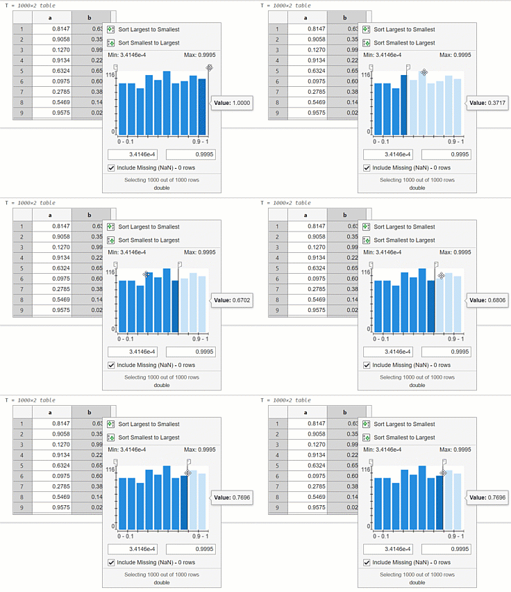
Live Editor: Improved performance when filtering numeric table variables
In the output of the Live Editor, the performance of filtering a numeric table or timetable variable is improved. When dragging the maximum or minimum value slider, the drag interaction is smoother and faster in R2023a than in R2022b, and the data tip displaying the current slider value appears to the side of the filtering figure.
For example, for a table output in the Live Editor, pause on the header of a numeric variable and click the triangle icon. Then, to filter the data, adjust the maximum value by dragging the slider. The drag interaction is smoother and tracks your mouse motion more closely in R2023a than in the previous release.
| R2022b | R2023a |
|---|---|
After dragging the maximum value slider in a filtering figure, the slider takes a moment to reposition and jumps to the new location. The associated data tip moves with the slider and obscures the filtering figure.
| After dragging the maximum value slider in a filtering figure, the slider follows the mouse motion more closely and repositions more quickly at the new location. The associated data tip is located in a fixed position to the right of the filtering figure.
|
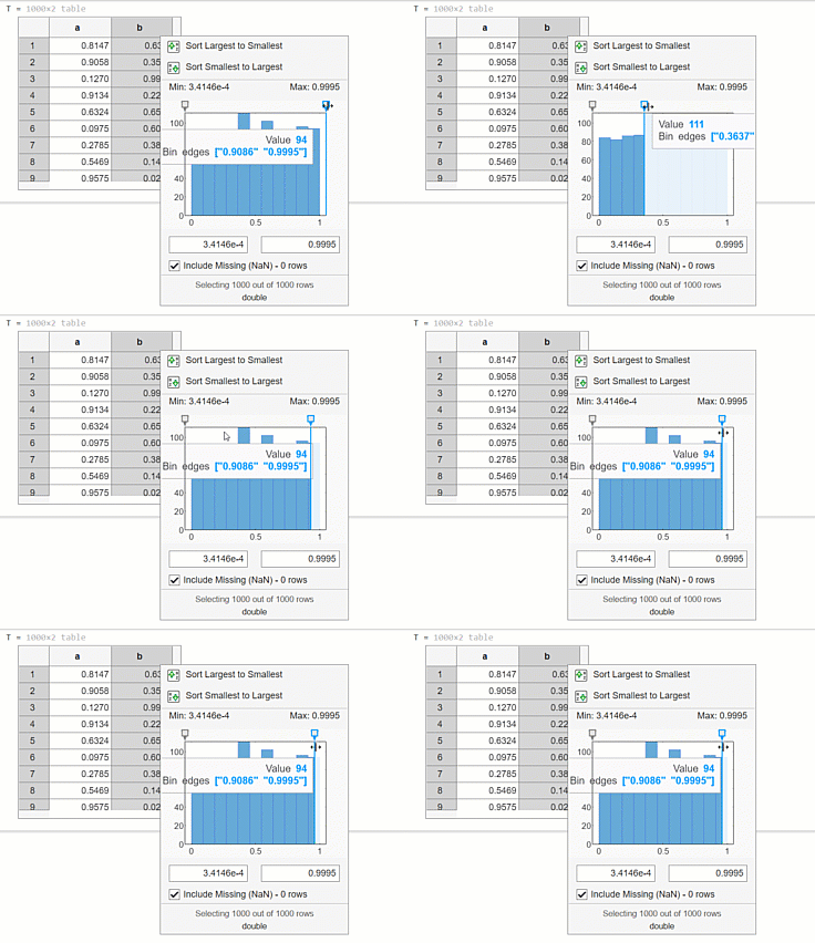
The filtering interaction was performed on a Windows 10, Intel Xeon CPU E5-1650 v4 @ 3.60 GHz test system by dragging the maximum value slider in the filtering figure for a 1000-row numeric table variable.
Property Inspector: Improved performance when opening for the first time
The Property Inspector shows improved performance when opening for the first time in a
MATLAB session. The delay between clicking the Property Inspector icon or calling
inspect and the inspector being ready is reduced.
For example, open the Property Inspector for the first time in a MATLAB session. You can use the Property Inspector 1.17x sooner than in the previous release.
ax = axes; inspect(ax)
The approximate rendering times are:
R2022b: 13.5 s
R2023a: 11.5 s
The rendering of the Property Inspector was timed on a Windows 10, Intel Xeon CPU E5-1650 v4 @ 3.60 GHz test system by running the code and measuring the time it takes for the edit fields to appear in the Property Inspector.
Property Inspector: Improved performance when switching between objects
The Property Inspector shows improved performance when switching between objects. The delay between selecting a different object and an existing instance of the Property Inspector rendering the properties of the newly selected object is reduced.
For example, open the Property Inspector. Then, create and inspect an
Axes object. The axes properties render 1.7x faster than in the
previous release.
inspect ax = axes; inspect(ax)
The approximate times for the Property Inspector to render the properties of the axes are:
R2022b: 3.5 s
R2023a: 2.1 s
The rendering of the Property Inspector was timed on a Windows 10, Intel Xeon CPU E5-1650 v4 @ 3.60 GHz test system by running the code and measuring the time it takes for the Property Inspector to be ready.
Variables Editor: Improved performance of cell editing in MATLAB Online
In the MATLAB Online Variables editor, when you interactively edit the value of a cell, the cell updates to display the new value more quickly in R2023a than in R2022b.
For example, create a 1000-element cell array and open the cell array in the Variables editor.
C = cell(1000);
openvar C
Then, double-click on a cell and enter a new value. On a Windows 10, Intel Xeon CPU E5-1650 v4 @ 3.60 GHz test system, when you move the focus from the edited cell, the cell value updates immediately. In R2022b, the cell value updates after a 3.5-second delay.
Variables Editor: Improved speed of data display when scrolling in MATLAB Online
In the MATLAB Online Variables editor, the performance of vertical and horizontal scrolling is improved. When scrolling within 1000 rows below the current element or 100 variables to the right of the current element, the data appears more quickly in R2023a than in R2022b.
For example, create a 1000-by-1000 matrix and open the matrix in the Variables editor.
X = rand(1000);
openvar XWhen you scroll down 100 rows, the values of all visible matrix elements in the Variables editor are rendered about 6.7x faster than in the previous release.
The approximate times for the Variables editor to render the values of all visible matrix elements are:
R2022b: 1.80 s
R2023a: 0.27 s
This interaction was timed on a Windows 10, Intel Xeon CPU E5-1650 v4 @ 3.60 GHz test system by running the above script and scrolling in the Variables editor.
App Building: Improved app startup performance
Apps created in App Designer and using the uifigure function
start up faster in R2023a than in R2022b and previous releases. The improvement is more
noticeable for apps with many UI components.
For example, this code creates an app with 1000 edit field components. The code is about 1.5x faster than in the previous release and about 3x faster than in R2021b.
function timingApp fig = uifigure; gl = uigridlayout(fig,Scrollable="on"); gl.RowHeight = repmat({'fit'},1,100); gl.ColumnWidth = repmat({'fit'},1,10); for k = 1:1000 uieditfield(gl); end end
The approximate execution times are:
R2021b: 21.5 s
R2022b: 10.6 s
R2023a: 7.2 s
The code was timed on a Windows 10, Intel
Xeon CPU E5-1650 v4 @ 3.60 GHz test system by running the
timingApp function and measuring the time it takes for the edit
fields to appear in the UI figure window.
App Building: Improved startup performance for apps with multiple tabs
In addition to the overall app startup performance improvement in R2023a, some apps that contain multiple tabs show an even greater startup performance improvement. The reason is that MATLAB prioritizes creating the content in the visible tab over non-visible content when the app first runs.
The particular performance improvement that you see depends on the app layout and UI component types. The improvement is more noticeable for apps with these types of UI components in unselected tabs:
Labels and spinners with a grid layout manager
Table UI components without a grid layout manager
For example, this code creates a tab group with five tabs, each containing 200 label components. The code is about 1.9x faster than in the previous release.
function timingTabApp fig = uifigure; tg = uitabgroup(fig); for k1 = 1:5 t = uitab(tg); gl = uigridlayout(t,Scrollable="on"); gl.RowHeight = repmat({'fit'},1,20); gl.ColumnWidth = repmat({'fit'},1,10); for k2 = 1:200 uilabel(gl); end end end
The approximate execution times are:
R2022b: 9.8 s
R2023a: 5.2 s
The code was timed on a Windows 10, Intel
Xeon CPU E5-1650 v4 @ 3.60 GHz test system by running the
timingTabApp function and measuring the time it takes for the
components to appear in the UI figure window.
If you have an app with many UI components, consider updating your app layout to take advantage of this improvement. For more information, see Improve App Startup Time.
When an app user switches to a new tab for the first time after running an app, the interaction might take more time than in previous releases. The reason is that MATLAB might create some content in the tab only after the user selects the tab. If the user later switches to the same tab again, the interaction does not take the additional time.
App Building: Improved performance when resizing some apps
When a user resizes an app figure window, some apps reposition their content faster in R2023a than in R2022b. The types of apps that show this improvement are:
Large apps with tabs that have an AutoResizeChildren
value of 'on'
Large apps with panels and button groups that have a
SizeChangedFcn callback
For example, this code creates an app with a tab group where each tab contains many edit fields that are resized automatically. The resize operation is smoother and faster in R2023a than in the previous release.
function tabResize fig = uifigure; tg = uitabgroup(fig,"Position",[20 20 400 375]); for k1 = 1:5 t = uitab(tg,"Scrollable","on"); for k2 = 1:100 ef = uieditfield(t,"Position",[50 22*k2 250 20]); end end end
| R2022b | R2023a |
|---|---|
When the app resizes, the app content takes multiple seconds to reposition. | When the app resizes, the app content takes less than one second to reposition. |
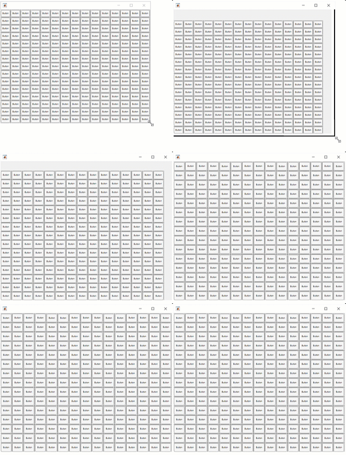
As another example, this code creates an app with many panels, each of which resizes a
button using a SizeChangedFcn callback whenever the app size changes.
The resize operation is smoother and faster in R2023a than in the previous
release.
function panelResize fig = uifigure("AutoResizeChildren","off", ... "SizeChangedFcn",@resizePanels); for k = 1:225 p = uipanel(fig, ... "AutoResizeChildren","off", ... "SizeChangedFcn",@resizeButtons); btn = uibutton(p,"Position",[2 2 20 20]); end end function resizeButtons(src,~) for k = 1:length(src.Children) src.Children(k).Position(3:4) = 0.9*src.Position(3:4); end end function resizePanels(src,~) xscale = src.Position(3)/15; yscale = src.Position(4)/15; for k = 1:length(src.Children) p = src.Children(k); p.Position = [xscale*(mod((k-1),15)), ... yscale*(floor((k-1)/15)), ... xscale, ... yscale]; end end
| R2022b | R2023a |
|---|---|
When the app resizes, the app content takes multiple seconds to reposition.
| When the app resizes, the app content takes about one second to reposition.
|
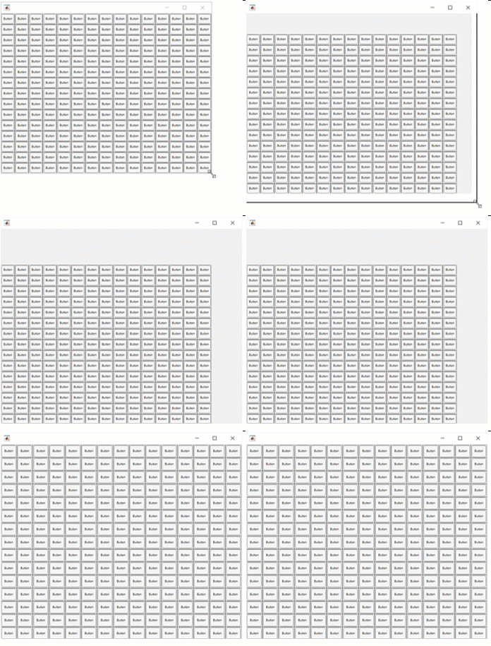
The resize interactions were performed on a Windows 10, Intel
Xeon CPU E5-1650 v4 @ 3.60 GHz test system by running the
tabResize and panelResize functions and
resizing the figure window.
Build Automation: Improve build speed and efficiency with incremental builds
The build tool supports incremental builds. Incremental builds avoid redundant work by skipping tasks that are up to date. If you want the build tool to skip a task when it is up to date, specify the inputs or outputs of the task. The build tool keeps track of the inputs and outputs every time the task runs and skips the task if they have not changed. For more information, see Improve Performance with Incremental Builds.
Build Automation: Create and run tasks that accept arguments
The build tool lets you create and run tasks that accept arguments. You can use task arguments to customize the actions that tasks perform when they run. For more information, see Create and Run Tasks That Accept Arguments.
Dependency Analyzer: Analyze files and folders with or without a project
Starting in R2023a, you can access Dependency Analyzer from the MATLAB apps gallery. You can now perform a dependency analysis on files and folders that do not belong to a project. For more information, see Dependency Analyzer.
Project Preferences: Recreate empty project folders in Git repositories
Git™ does not track empty folders and ignores them when you commit. MATLAB now enables you to recreate an empty folder structure in a project under Git source control. Doing so is useful for small projects intended for training or as procedure templates.
For large projects, to avoid performance issues on startup, clear Recreate empty project folders in a project under Git. For more information, see Set MATLAB Projects Preferences.
Project API: Determine if file is under project root folder
You can now programmatically determine whether a file or a folder is under a project
root folder by using the matlab.project.isUnderProjectRoot function.
Project API: Export subset of project files to archive
You can now programmatically export a subset of project files to an archive by specifying a user-defined export profile in the export function.
Project Sharing: Include only specific files in project archive using export profile
You can now use an export profile to include only files with particular labels in a project archive. This option is useful if the files you need to share are only a small subset of a large project. For more information, see Create an Export Profile.
Comparison Tool: Automate comparison report generation for continuous integration (CI) workflows
Starting in R2023a, you can programmatically publish comparison reports for plain text
files, MATLAB scripts, and text-based source code files. Automate report generation for
continuous integration (CI) workflows using the visdiff
function.
comparison = visdiff(textfile1,textfile2); file = publish(comparison); web(file)
Source Control in MATLAB Online: Save uncommitted changes by creating a Git stash
In MATLAB Online, you can now save uncommitted changes by creating a Git stash.
Source Control in MATLAB Online: Manage Git remote repositories locally using Branch Manager
In MATLAB Online, you can now manage multiple remote repositories from a local Git repository. Use Branch Manager to perform these tasks:
Add, edit, and delete remote repositories.
Fetch from all remotes or individual remotes.
Prune remote branches from all or individual remotes.
Open selected remotes in a web browser.
Create new local branches that track remote branches.
Delete remote branches.
Source Control in MATLAB Online: Detect and extract conflict markers from text and binary files
In MATLAB Online, you can now detect conflict markers added by Git in text and binary files. Extract conflict markers to repair corrupted files.
Comparison Tool in MATLAB Online: Compare project definition files
Starting in R2023a, when you compare folders in MATLAB
Online, MATLAB detects whether they are project root folders. MATLAB looks for and compares the project definition files stored in the
resources or .SimulinkProject folder. Project
definition files contain information about the project path, project settings,
shortcuts, labels, and referenced projects. For more information, see Compare MATLAB Projects in MATLAB
Online.
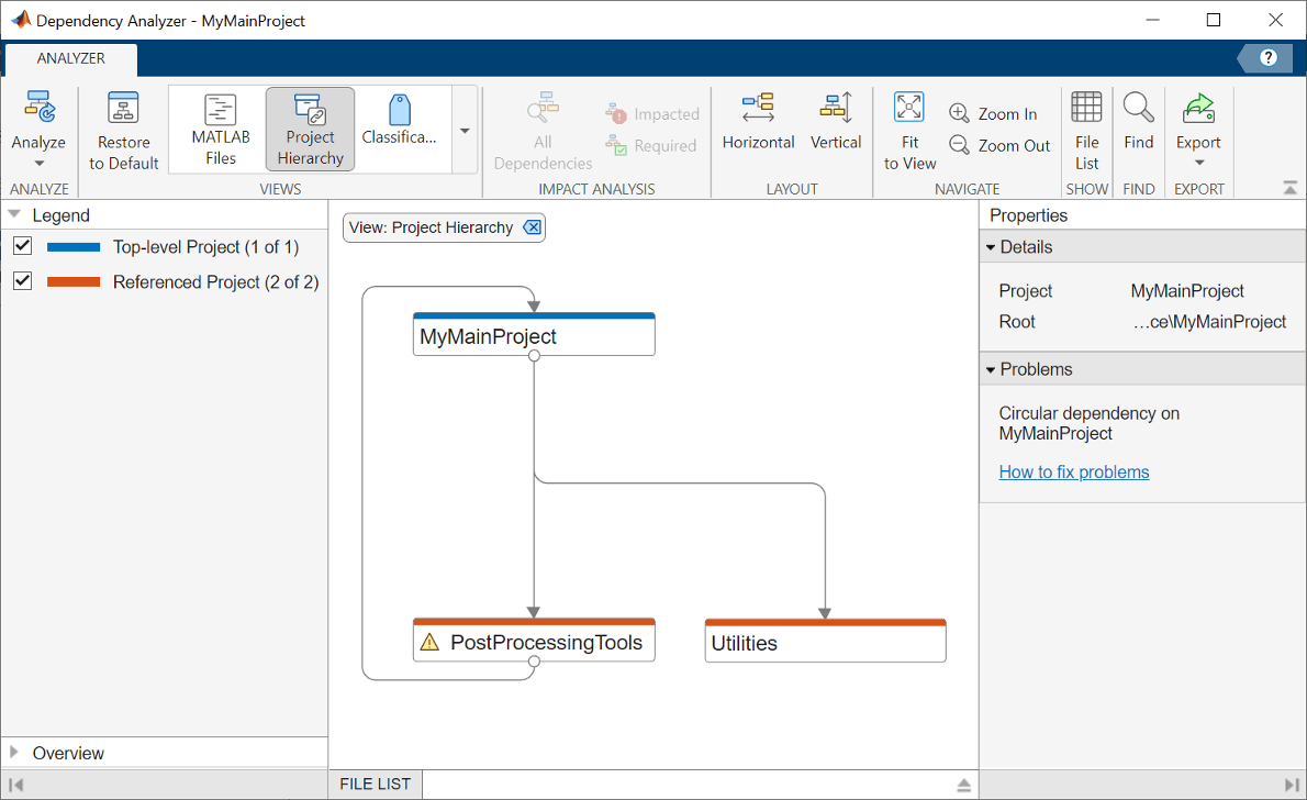
Dependency Analyzer in MATLAB Online: Investigate circular dependencies using the Project Hierarchy view
You can now investigate how projects in your hierarchy relate to each other and identify projects that introduce circular dependencies using the Project Hierarchy view in MATLAB Online. For more information, see Analyze Project Dependencies.
Unit Testing Framework: Run tests interactively by using Test Browser
The Test Browser app enables you to run script-based, function-based, and class-based tests interactively. You can use the test browser to:
Create a test suite from files and folders.
Run all or part of the specified tests.
Access diagnostics and debug test failures.
Customize a test run with options, such as running tests in parallel (requires Parallel Computing Toolbox™) or specifying a level of test output detail.
Generate an HTML code coverage report for MATLAB source code.
For more information, see Run Tests Using Test Browser.
Unit Testing Framework: Programmatically access code coverage results
You can use the matlab.unittest.plugins.codecoverage.CoverageResult class to
programmatically access the results of code coverage analysis for your source code. To
generate and access the coverage results, create a CodeCoveragePlugin instance using a CoverageResult object,
and add the plugin to the test runner. After the test run, the
Result property of the CoverageResult object
holds the coverage results as an array of matlab.coverage.Result objects. Each element of the array provides
information about one of the files in your source code that was covered by the
tests.
For more information, see Collect Statement and Function Coverage Metrics for MATLAB Source Code.
Unit Testing Framework: Temporarily set environment variables
The matlab.unittest.fixtures.EnvironmentVariableFixture class provides a
fixture for setting an operating system environment variable. Once the testing framework
tears down the fixture, the fixture restores the environment variable to its original
state.
Unit Testing Framework: Test for handle validity
The matlab.unittest.constraints.IsValid class provides a constraint to test if
a handle array is valid. The constraint is satisfied if all array elements are valid
handles.
Unit Testing Framework: Write text to files in thread-based environment
You can use the ToFile and ToUniqueFile
classes in a thread-based environment to write text to UTF-8 encoded files.
Unit Testing Framework: Use renamed classes in testing and other automated workflows
To reflect support for additional automated workflows, a group of
matlab.unittest classes have been renamed. For example,
matlab.unittest.Verbosity is now named
matlab.automation.Verbosity.
This table shows the affected classes and their new names. The behavior of these classes remains the same, and existing instances of these classes in your code continue to work as expected. There are no plans to remove support for existing instances of these classes.
| R2022b and Earlier | Starting in R2023a |
|---|---|
matlab.unittest.Verbosity | matlab.automation.Verbosity |
matlab.unittest.diagnostics.Diagnostic | matlab.automation.diagnostics.Diagnostic |
matlab.unittest.diagnostics.DiagnosticResult | matlab.automation.diagnostics.DiagnosticResult |
matlab.unittest.diagnostics.DisplayDiagnostic | matlab.automation.diagnostics.DisplayDiagnostic |
matlab.unittest.diagnostics.FileArtifact | matlab.automation.diagnostics.FileArtifact |
matlab.unittest.diagnostics.FunctionHandleDiagnostic | matlab.automation.diagnostics.FunctionHandleDiagnostic |
matlab.unittest.diagnostics.StringDiagnostic | matlab.automation.diagnostics.StringDiagnostic |
matlab.unittest.plugins.OutputStream | matlab.automation.streams.OutputStream |
matlab.unittest.plugins.ToFile | matlab.automation.streams.ToFile |
matlab.unittest.plugins.ToStandardOutput | matlab.automation.streams.ToStandardOutput |
matlab.unittest.plugins.ToUniqueFile | matlab.automation.streams.ToUniqueFile |
App Testing Framework: Test context menus within labels
You can use the chooseContextMenu method to test a right-click that opens a context menu
within label components. For example, assign a context menu with two items to a label,
and then choose the first menu item.
fig = uifigure; lbl = uilabel(fig); cm = uicontextmenu(fig); m1 = uimenu(cm,Text="Menu1"); m2 = uimenu(cm,Text="Menu2"); lbl.ContextMenu = cm; testCase = matlab.uitest.TestCase.forInteractiveUse; testCase.chooseContextMenu(lbl,m1)
Performance Testing Framework: Use fewer samples to meet the objective margin of error
The default number of times that the framework exercises the test code to warm it up
in a frequentist time experiment (created using either the runperf function or the limitingSamplingError static method) has increased from four to five. This
change results in typically fewer samples required to meet the objective relative margin
of error.
If your code relies on the previous default value, you might need to update your
code. For example, if you use warmupTable =
results(1).TestActivity(1:4,:) to create a table of warm-up
measurements, replace 4 with 5. Also, if you
want to keep using the previous default value, explicitly specify the value in your
code. This table shows an example of how to update code that runs tests using four
warm-up measurements.
| Before | After |
|---|---|
import matlab.perftest.TimeExperiment
experiment = TimeExperiment.limitingSamplingError;
results = run(experiment,mySuite); |
import matlab.perftest.TimeExperiment experiment = TimeExperiment.limitingSamplingError("NumWarmups",4); results = run(experiment,mySuite); |
Functionality being removed or changed
TaskAction constructor method has been removed
Errors
The constructor method of the matlab.buildtool.TaskAction class has been removed. To specify a task
action, use a function handle instead of the constructor method. This table shows an
example of how to update code that calls the TaskAction constructor
method.
| Before | After |
|---|---|
import matlab.buildtool.Task import matlab.buildtool.TaskAction plan = buildplan; plan("test") = Task( ... Actions=TaskAction( ... @(~)assertSuccess(runtests(IncludeSubfolders=true)),Name="Testing")); |
import matlab.buildtool.Task plan = buildplan; plan("test") = Task( ... Actions=@(~)assertSuccess(runtests(IncludeSubfolders=true))); |
Publish C++ Interface: Publish interface for C++ library in Live Editor
The clibPublishInterfaceWorkflow function creates a live script that guides
you through the steps to publish a MATLAB interface to a C++ library. For more information, see Steps to Publish a MATLAB Interface to a C++ Library and
Generate C++
Interface.
Interface to C++ Library: Execute C++ library functions out-of-process
Run C++ library functions in processes that are separate from the MATLAB process. For more information, see Load C++ Library In-Process or Out-of-Process. Use out-of-process mode to call functions in third-party libraries that are not compatible with MATLAB. Publishers can use this mode while developing an interface, eliminating the need to restart MATLAB while testing.
Interface to C++ Library: Support for default arguments
If a C++ function is defined with default arguments, then you can call the function without providing one or more trailing arguments. MATLAB supports default arguments for scalar integer and floating-point types.
The MATLAB interface to C++ libraries displays default arguments in function
signatures in the library definition file and in the help text. For example, the
argument arg for the function funcname has a
default value of 5.
% C++ Signature: void funcname(double arg = 5.000000)
These calls to funcname produce the same result:
clib.libname.funcname clib.libname.funcname(5)
For more information, see Call Function with Default Arguments.
Interface to C++ Library: Support for comments in function templates
The generated help text in a MATLAB interface to a C++ library includes Doxygen comments from template functions and template methods of a class. For information about viewing these comments, see Display Help for MATLAB Interface to C++ Library. For information about modifying comments when publishing an interface, see Publish Help Text for MATLAB Interface to C++ Library.
Publish C++ Interface: Put libraries on run-time path
Use the copyRuntimeDependencies function to copy dependent libraries to the
run-time path so that they are available when you test. This function collects the
necessary files for distributing to end users so that they do not have to set
environment variables to call functions in the library. For information, see Set Up and Copy Run-Time Libraries.
Publish C++ Interface: Resolve multiple redefinition and unresolved external symbol errors
Error messages for multiple redefinition and unresolved external symbol compiler errors provide additional help for you to resolve the error. For more information, see Resolve Build Error: Multiple Redefinition Linker Errors and Resolve Build Error: Unresolved External Symbols.
Publish C++ Interface: Information to debug C++ library functions
You can debug C++ library functions by using a debug-version of the MATLAB interface to the library. For steps to build a debug-version, see Debug C++ Library from MATLAB Interface.
Publish C++ Interface: Support for MATLAB operators for C++ methods
In a MATLAB interface to a C++ library, MATLAB operators are supported when corresponding methods are defined in a C++ class.
Operation in MATLAB | Method to Define in C++ Class |
|---|---|
a < b | lt(a,b) |
a > b | gt(a,b) |
a <= b | le(a,b) |
a >= b | ge(a,b) |
a ~= b | ne(a,b) |
a == b | eq(a,b) |
Java Interface: Support for Java 11 JDK and JRE
MATLAB supports Java 11 JDK™ and JRE™. To use this version, located in the folder jre_path,
call the jenv
function. At the MATLAB prompt, type:
e = jenv("jre_path")You might have to restart your MATLAB session to change to this version.
Java Interface: jenv and matlab_jenv
provide environment information
The jenv
function returns a JavaEnvironment object, which contains information about the Java program on your system. The matlab_jenv command displays Java environment information at the operating system prompt, but it does not
return the information.
Python Interface: Convert between MATLAB
datetime and Python
datetime, NumPy datetime64 types
You can convert between MATLAB
datetime values and Python®
datetime or NumPy datetime64 values. For examples,
see Use MATLAB
datetime Types with Python.
Python Interface: Convert between MATLAB
duration and Python
timedelta, NumPy timedelta64 types
You can convert between MATLAB
duration values and Python
timedelta or NumPy timedelta64 values. For
examples, see Use MATLAB
duration Types with Python.
Python Objects: Use Python objects as keys in dictionary
You can use Python objects as keys in dictionaries. For more information about dictionary keys, see dictionary.
.NET Interface: Convert between MATLAB dictionary and .NET
System.Collections.Generic.Dictionary objects
You can convert a MATLAB dictionary to a .NET dictionary. For more information, see Pass Data to .NET Objects.
To explicitly create a .NET dictionary from a MATLAB dictionary, call the NET.createDictionary function.
To convert a .NET dictionary to a MATLAB dictionary, see How MATLAB Handles .NET Dictionary Objects.
.NET Objects: Use .NET objects as keys in dictionary
You can use .NET objects as keys or values in dictionaries. For more information about dictionary keys, see dictionary.
.NET Engine: Support for MATLAB structs
Use the .NET MathWorks.MATLAB.Types.MATLABStruct class to represent MATLAB struct objects. For examples, see Use MATLAB Structures in .NET.
Perl 5.36.0: MATLAB support on Windows
As of R2023a, MATLAB on Windows ships with an updated version of Perl, version 5.36.0, and supports an updated version of HTML::Parser, version 3.78.
If you use the perl command on Windows platforms, see https://www.perl.org/ for information about using this version of the Perl programming
language. For a standard distribution of HTML::Parser, source code, and information
about using HTML::Parser, see https://metacpan.org/pod/HTML::Parser.
Compiler support changed for building C and C++ interfaces, MEX files, and standalone MATLAB engine and MAT-file applications
| Support | Compiler | Platform |
|---|---|---|
Added | Intel oneAPI 2023 with Microsoft® Visual Studio® 2019 and 2022 for C, C++, and Fortran | Windows |
Added | Intel oneAPI 2022 with Microsoft Visual Studio 2017, 2019, and 2022 for C, C++, and Fortran | Windows |
Added | MinGW®-w64 version 8.1 compiler. For installation instructions, see this MATLAB Answers™ article FAQ: How do I install the MinGW compiler? | Windows |
To be phased out | Intel Parallel Studio XE for C/C++ | Windows |
For continued support for building your applications, consider upgrading to a supported compiler. For an up-to-date list of supported compilers, see Supported and Compatible Compilers.
Functionality being removed or changed
Python version 2.7 is no longer supported
Errors
Support for Python version 2.7 is discontinued. For continued support for your applications, upgrade to a supported version of Python. For supported version information, see Versions of Python Compatible with MATLAB Products by Release.
-std=c++11 flag is no longer included in MEX options
files
Behavior change
MEX options files for building C++ code with MinGW and Linux® compilers no longer include the CXXFLAGS option
-std=c++11.
MEX options files for macOS compilers include the CXXFLAGS option
-std=c++14 instead.
However, you can still build MEX files with the -std=c++11
option. For example, build the MEX file myFunc.cpp with that
option.
mex myFunc.cpp 'CXXFLAGS=$CXXFLAGS -std=c++11'
Continuous console and writer output for MATLAB API for Java functions
Behavior change
When you call a MATLAB function that displays output using one of the evaluate functions in
com.mathworks.engine.MatlabEngine,
then the output continuously displays on the console and writer output stream. This
behavior applies to feval, fevalAsync,
eval, and evalAsync.
Before R2023a, the output displays after the MATLAB function completes.
.NET Interface: Dictionary with cell types map to .NET
System.Object instead of
System.Object[]
Behavior change
A MATLAB dictionary with entries of type cell are converted
to a .NET dictionary with entries of type System.Object.
Previously, the conversion was to System.Object[]. For more
information, see Pass Data to .NET Objects and How MATLAB Handles .NET Dictionary Objects.
Support for MJPEG format in USB Webcams on Windows
Starting R2023a, the MATLAB Support Package for USB Webcams installed on a Windows machine supports the MJPEG image format. The MJPEG format provides improved frame rates for acquiring high-resolution images from a USB webcam.
Support for 32-bit Debian Bullseye on Raspberry Pi
Raspberry Pi® Blockset now supports 32-bit Debian® Bullseye for MATLAB desktop and MATLAB Online. You can now customize Debian Bullseye running on your Raspberry Pi hardware to make it compatible with MATLAB while doing the Hardware Setup.
Support for Raspberry Pi Zero 2 W and Raspberry Pi Compute Module 4
You can now use the Raspberry Pi Blockset with Raspberry Pi Zero 2 W and Raspberry Pi Compute Module 4 for MATLAB desktop and MATLAB Online.