Environment
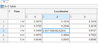
You can add tables to your live scripts and functions to format text and images. To
insert a table, go to the Insert tab and select
Table
![]() . Move the cursor over the grid to highlight the numbers
of rows and columns you want and then click to add the table. To create a larger table,
select the Insert a table button and specify the numbers of rows and columns in the dialog
box.
. Move the cursor over the grid to highlight the numbers
of rows and columns you want and then click to add the table. To create a larger table,
select the Insert a table button and specify the numbers of rows and columns in the dialog
box.
After inserting the table, to modify its rows and columns, right-click the table, select Table, and select from the available options. For more information, see Format Text in the Live Editor.
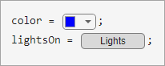
You can add a color picker to your live script to select a color interactively. You also can add a state button to indicate and interactively set the value of a logical variable.
To add a color picker, go to the Live Editor tab, and in the Code section, select Control > Color Picker. To add a state button, select State Button.
For more information, see Add Interactive Controls to a Live Script.
You can now use keyboard shortcuts to interact with inline output in live scripts. To move focus from the code to the output, use the down arrow and up arrow keys. To activate an output, press Enter. Once an output is activated, you can scroll text using the arrow keys, navigate through hyperlinks and buttons using the Tab key, and open the context menu by pressing Shift+F10. To deactivate an output, press Esc.
To disable using the keyboard to move focus to the output when output is inline, on the
Home tab, in the Environment section, click
![]() Preferences. Select MATLAB > Editor/Debugger > Display, and clear the Focus outputs using keyboard when output is
inline option.
Preferences. Select MATLAB > Editor/Debugger > Display, and clear the Focus outputs using keyboard when output is
inline option.
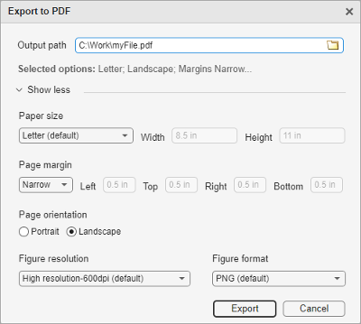
When exporting to PDF, Microsoft® Word documents, HTML, and LaTeX, you can use the Export dialog box to customize export options interactively. To open the Export dialog box, on the Live Editor tab, click Export and then select an export format. In MATLAB Online™, click Save instead of Export.
You can change the paper size, orientation, and margins when exporting to PDF, Microsoft Word documents, and LaTeX. You also can change the resolution and format of figures when exporting to PDF, HTML, and LaTeX (requires the files to be run before exporting).
For more information, see Ways to Share and Export Live Scripts and Functions.
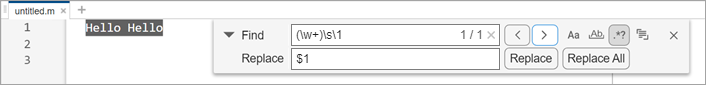
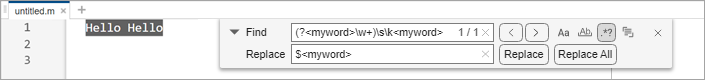
Search for and replace groups of characters in a file using capture groups in regular
expressions. To begin searching using regular expressions, on the Editor or Live Editor tab, in the Navigate section, click ![]() Find. Then, select the Regular expression option
Find. Then, select the Regular expression option
![]() .
.
To create a capture group, surround the characters that you want to group with
parentheses. Then, to access the capture group within the regular expression, use the
format \, where
numbernumber$. For example, to find duplicate
words in a file, use the expression number(\w+)\s\1. To replace the two words
with just one word, use the expression $1.
You also can create a named capture group using the format
?<, where
name>name\k< within the regular
expression, or name>$< within a
replacement pattern. For example, to find duplicate words using a named capture group, use
the expression name>(?<myword>\w+)\s\k<myword>. To replace the two
words with just one word, use the expression $<myword>.
For more information about searching using the find and replace dialog box, see Find and Replace Text in Files and Go to Location.
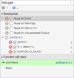
Use the Debugger panel to manage breakpoints and navigate the function call stack while
debugging in MATLAB
Online. To open the Debugger panel, go to the Editor or
Live Editor tab, and in the Analyze section,
click ![]() Debugger. You also can open the panel using the Open more panels
button (
Debugger. You also can open the panel using the Open more panels
button (![]() ) in the sidebar.
) in the sidebar.
For more information, see Debug MATLAB Code Files.
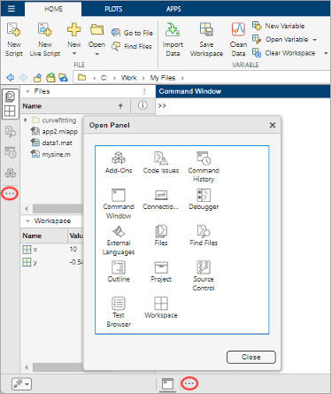
In MATLAB
Online, you can open additional panels (also referred to as tools) directly from the
sidebars. To open additional panels, in a sidebar, click the Open more panels button (![]() ). Then, in the Open Panel dialog box, select from the
available panels. You also can right-click in a sidebar and select Open more
panels.
). Then, in the Open Panel dialog box, select from the
available panels. You also can right-click in a sidebar and select Open more
panels.
For example, to open the Code Issues panel, click the Open more panels button (![]() ), and select the Code Issues panel.
), and select the Code Issues panel.
For more information, see Change Desktop Layout.
In MATLAB Online, when you click the MATLAB background, open windows in the foreground collapse. Collapsing a window reduces the size of the window by displaying only its title bar.
![]()
To restore the collapsed windows, click the title bar of one of the previously open windows.
To prevent a window from being collapsed or minimized, click ![]() on its title bar.
on its title bar.
For more information, see Manage Windows in MATLAB Online.
Language and Programming
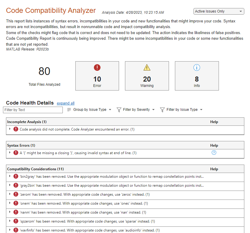
The Code Compatibility Analyzer app has a new interface that makes it easier to navigate issues found in code. You can now adjust how identified issues are grouped and filter results by text, severity, and issue type.
Data Analysis
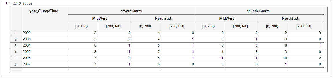
Starting in R2023b, the output of the Live Editor displays the contents of tables or timetables that contain nested tables or timetables as variables inline. You can interactively manipulate a nested table, for example, by selecting or sorting a variable or copying a variable with its headers. Previously, the output of the Live Editor displayed the dimensions of nested tables, but not the nested table contents.
For example, use the Pivot Table task to create nested tables. The Live Editor output displays the complete pivoted table contents.
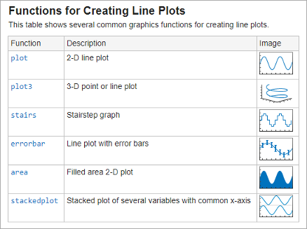
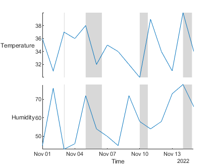
The stackedplot
function can plot events as lines or shaded regions on stacked plots created from
timetables. To plot events associated with a timetable, you must attach an event table to
it before you call stackedplot. For more information on event tables,
see eventtable.
To support events, stackedplot has a new
EventsVisible name-value argument:
If
EventsVisibleis"on", thenstackedplotplots events as lines or shaded regions.If
EventsVisibleis"off", thenstackedplothides events.
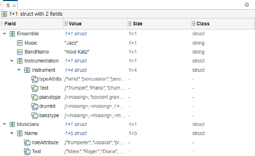
The Variables editor in MATLAB Online has improved functionality for these data types:
Scalar structure — You can now view, expand, and interactively edit the fields and nested fields in a scalar structure. Previously, you had to open each field in another tab in the Variables editor to view and edit its contents.
Object array — You can now view and interactively edit the values of common properties of objects in an object array. Previously, you had to open each object in a separate tab in the Variables editor to view and edit its property values.
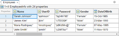
Table with grouped variables — You can now select and interactively edit the contents of a subcolumn in a group of table variables. Previously, interactively editing a subcolumn in a group of table variables was not supported.
Data Import and Export
Mathematics
You can change the default algorithm and seed for the rng function from the MATLAB Preferences window. On the Home tab, in the
Environment section, click ![]() Preferences. Select MATLAB > General, and then select a different option for Default
algorithm and select a different value for Default
seed in the Random Number Generation
preference.
Preferences. Select MATLAB > General, and then select a different option for Default
algorithm and select a different value for Default
seed in the Random Number Generation
preference.
To access and modify
settings for the random number generator programmatically, you can access the
matlab.general.randomnumbers settings using the root
SettingsGroup object returned by the settings
function. For example, show the default algorithm and seed that you have set for the random
number generator.
s = settings;
s.matlab.general.randomnumbers.DefaultAlgorithm
s.matlab.general.randomnumbers.DefaultSeed
When you first start a MATLAB session or call rng("default"), MATLAB initializes the random number generator using the default algorithm and seed
that you have set. If you do not change these settings, then rng uses
the factory value of "twister" for the Mersenne Twister generator with
seed 0, as in previous releases.
When you perform parallel processing (requires Parallel Computing Toolbox), by default, the MATLAB client uses the Mersenne Twister random number generator with seed 0 and the
MATLAB workers use the Threefry 4x64 generator with 20 rounds with seed 0. Changing
the default generator settings in the MATLAB Preferences window or using the
matlab.general.randomnumbers settings affects only the default
behavior of the client and does not affect the default behavior of the parallel
workers.
When using the rng function, you can specify just the algorithm for
the random number generator to use. The rng(generator) syntax allows you
to set the random number algorithm without specifying the seed, where
rng uses a seed of 0. This syntax is equivalent to
rng(0,generator). For example, rng("philox")
initializes the Philox 4x32 generator with a seed of 0.
Graphics
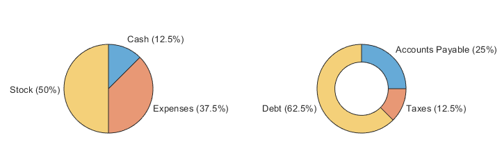
Use the piechart and
donutchart
functions to create charts with more configuration options and interactivity than pie
charts had in previous releases.
Some of the improvements include:
More options for formatting slice labels, slice placement, and colors
Data tips that appear when you move the cursor over the slices
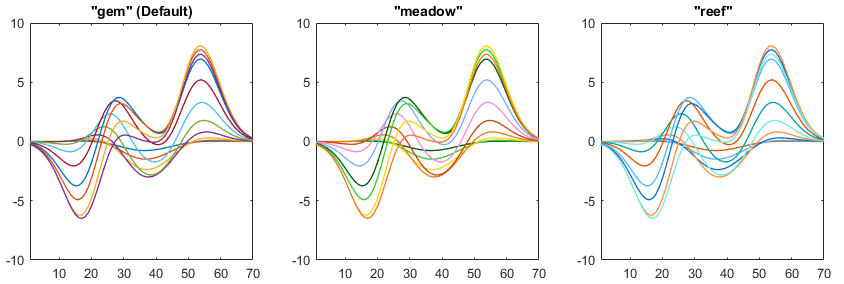
Plot multiple data series together using one of nine different color palettes to
differentiate the individual data series. You can change the palette by passing the
palette's name to the colororder
function. The available names are "gem", "gem12",
"glow", "glow12", "sail",
"reef", "meadow", "dye", and
"earth". The "gem" palette is the default for most
plots.
You can also use the orderedcolors
function to get the RGB triplets for any of the palettes.
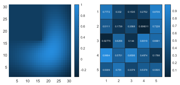
Use the abyss
function to get a blue-to-black colormap for coloring your charts. Like for all predefined
colormaps, you can optionally specify the number of colors for the abyss colormap.
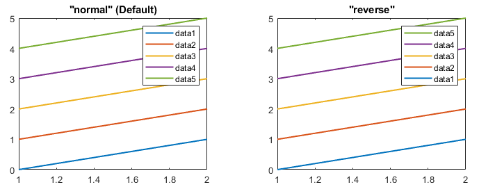
Control the order of legend entries by setting the Direction
property of the legend to "normal" or "reverse". In
most cases, the default direction is "normal".
Legends for stacked bar charts and area charts have a reverse order by default so the legend entries match the stacking order of the chart. For more information, see Legend order is reversed for stacked bar charts and area charts.
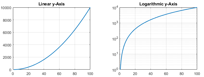
View any dimension of a plot on a logarithmic or linear scale by calling the xscale,
yscale, or
zscale
function after plotting. To switch between the different scales, call any of these
functions with "linear" or "log" as an input
argument. For example, yscale("log") changes the scale of the
y-axis to be logarithmic.
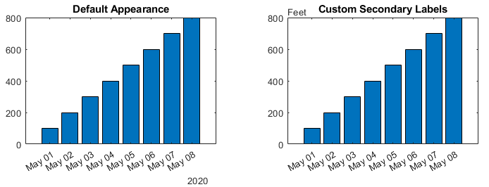
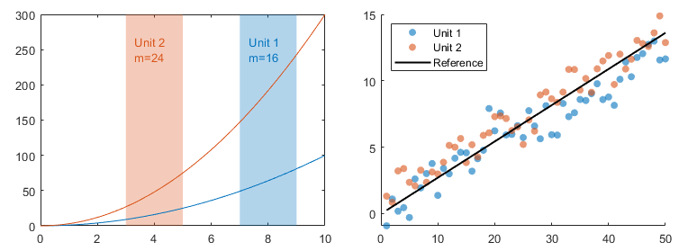
Create, delete, or modify secondary axis labels by calling the xsecondarylabel, ysecondarylabel, and zsecondarylabel functions. Secondary labels are text labels that appear at
the edge of the axes and provide additional information about the data. Often, they provide
information about the units or scale of the data.
For example, create a bar chart with datetime values along the x-axis
and feet along the y-axis. By default, the chart has a secondary
x-axis label of "2020". Call the
xsecondarylabel function with an empty string to delete the
"2020" label. Then add a secondary label of "Feet"
to the y-axis.
x = datetime(2020,5,1:8);
y = 100:100:800;
bar(x,y)
xsecondarylabel("");
ysecondarylabel("Feet")
Create unbounded filled regions by passing Inf or
-Inf to the xregion and
yregion
functions. You can also create multiple regions by specifying one matrix input argument as
an alternative to specifying two vectors of coordinates. For n regions,
the matrix must be 2-by-n or n-by-2 and contain the
lower and upper bounds for all the regions.
Create text objects with the anchor point positions included in the axes limits
calculation. To include an anchor point in the calculation, set the AffectAutoLimits property of the text object to
"on".
For example, create a line plot.
x = 0:0.1:10;
y = sin(x);
plot(x,y)
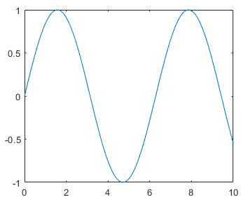
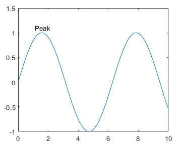
Create a text object outside of the current y-axis limits. Set the
AffectAutoLimits property to "on" so that the
axes limits adjust to include the anchor point of the text.
text(1.1,1.1,"Peak",AffectAutoLimits="on")
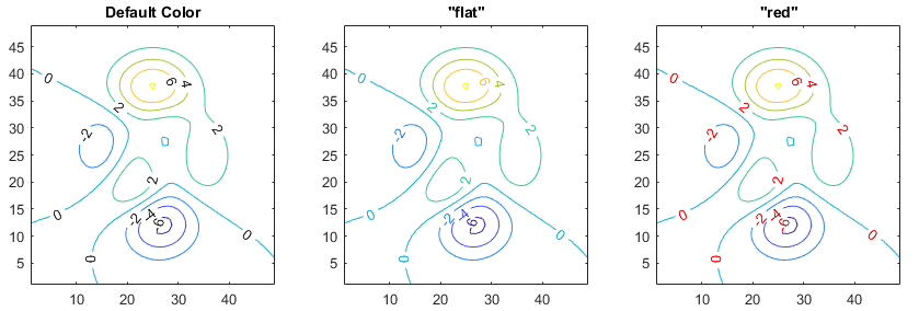
Set the LabelColor
property of a Contour object to display labels that match the colors of
the contour lines, or specify one color for all the labels.
Now you can match the colors and line styles of more objects in the axes by setting the
SeriesIndex property of the objects to the same value. The
SeriesIndex property is available for Text,
ConstantLine, ConstantRegion,
Rectangle, Patch, and
AnimatedLine objects, and lines created by the line, streamline, and streamslice functions.
Also, the SeriesIndex property has a new option,
"none", which enables you to opt out of automatic selection for
certain objects, such as reference lines.
With the new SeriesIndex property support, lines created with the
line, streamline, and
streamslice functions have a different default color. For more
information, see Default color is different for lines created with the line
function and Default color is different for plots created with the streamslice
and streamline functions.
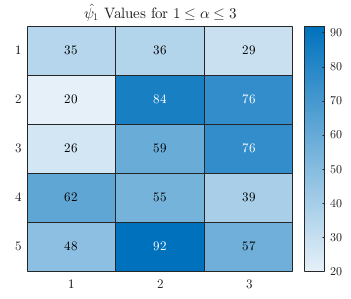
Create text, such as titles and axis labels, for heatmap charts with TeX markup, LaTeX markup, or no markup by setting the
Interpreter
property of the chart.
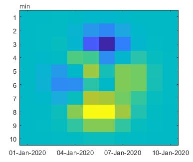
You can now display images using datetime, duration, or categorical coordinate values
with the image and imagesc functions. Previously, only numeric and logical coordinate values
were supported.
For example, display an image with datetime values along the x-axis and duration values along the y-axis.
x = datetime(2020,1,[1 10]);
y = minutes([1 10]);
C = peaks(10);
imagesc(x,y,C)
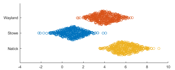
Create a horizontal swarm chart by setting the YJitter property
when you call the swarmchart
function. When you specify the YJitter property without specifying the
XJitter property, MATLAB sets the XJitter property to "none",
and the resulting distributions in the chart are horizontal.
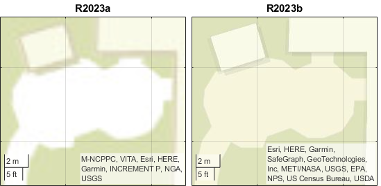
The "streets-light", "streets-dark",
"streets", and "topographic" basemaps hosted by
Esri®, which are used by geographic axes objects and other objects with a
Basemap property, have an improved visual appearance at high zoom
levels. For example, this image compares a basemap at zoom level 21 in R2023a with the same
basemap and zoom level in R2023b.
The basemaps can also have different appearances at other zoom levels. For example, this image compares a basemap at zoom level 15 in R2023a with the same basemap and zoom level in R2023b.
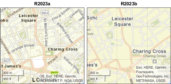
For more information about changing the basemap of geographic axes, see geobasemap.
The basemaps hosted by Esri update periodically. As a result, you might see differences in your visualizations over time.
The default order of legend entries for stacked (vertical) bar charts and area charts is now reversed to match the stacking order of the chart. Previously, the legend entries were listed in the opposite order of stacked bars and area charts.
To preserve the order of previous releases, set the Direction
property of the legend to "normal".
lgd = legend;
lgd.Direction = "normal";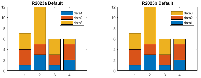
Now that the SeriesIndex property is available for lines created
with the line function, the lines cycle through the
same colors (and optional line styles) that most other plots do.
The default color change applies only to the lines you create when you specify the
x, y, and optional z
arguments. If you create lines with a syntax that uses name-value arguments only, the
plots look the same as in previous releases.
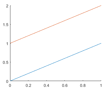
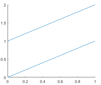
For example, create two lines with x and y input arguments. In R2023b, the first line is blue and the second line is red-orange. Before R2023b, both lines were blue.
line1 = line([0 1],[0 1]);
line2 = line([0 1],[1 2]);
To preserve the behavior of previous releases, set the
SeriesIndex property of the lines to 1. You
can set the property using a name-value argument when you call the
line function, or you can set the property of the
Line object using dot notation later.
% Use a name-value argument
line1 = line([0 1],[0 1],SeriesIndex=1);

% Use dot notation
line2 = line([0 1],[1 2]);
line2.SeriesIndex = 1;
When you create a streamslice or streamline plot, MATLAB automatically assigns colors and line styles the same way as for most
other plots. For example, the first set of lines created with
streamslice are now a soft blue color.
[x,y] = meshgrid(-10:10);
u = 2.*x.*y;
v = y.^2 - x.^2;
slicelines = streamslice(x,y,u,v);
axis tight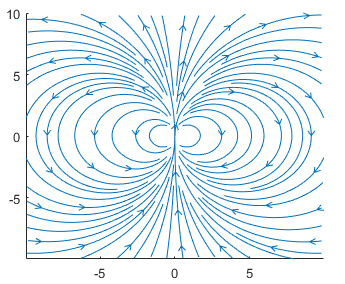
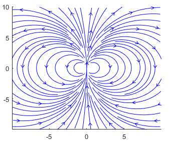
If you call either of the functions repeatedly, subsequent plots cycle through the same set of colors as other plots do. In previous releases, the lines were bright blue.
To preserve the appearance from previous releases, use the set
function to set the Color property to [0 0
1].
set(slicelines,Color=[0 0 1])
App Building
You can create a range slider using the uislider function by specifying the style as "range".
Alternatively, in App Designer, you can drag a Slider (Range)
component from the Component Library onto the canvas. The range slider
has two thumbs that app users can use to adjust the range of values. For example, this code
creates a range slider that specifies values from 10 to 60.
fig = uifigure;
sld = uislider(fig,"range",Value=[10 60]);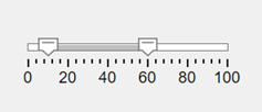
Interactively rearrange tabs, menus, tree nodes, and toolbar tools between parents by dragging the component in the Component Browser. For example, interactively move and change the parents of menus and menu items.
For a 2-D view of a 3-D chart in apps created in App Designer or using the
uifigure function, you can zoom into a rectangular region. To
enable region-zooming, click the Zoom In or Zoom Out button in the axes toolbar, or set the
Interactions property of the axes to the
regionZoomInteraction object.
For example, create a 3-D surface plot and set the view to the x- and z-axes. Click the Zoom In button and then drag to select the region of interest.
f = uifigure;
a = axes(f);
surf(a,peaks);
view(a,[0 0]);
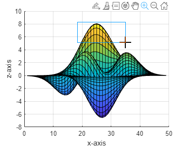
Previously, for 3-D charts, the region-zoom interaction was supported only for the xy view.
Performance
Tiled chart layouts that have the "flow" tile arrangement and axes
that span many tiles are more responsive when the tile arrangement changes. The tile
arrangements change under these conditions:
Adding new axes
Resizing the figure
Customizing the appearance of the axes by setting axes properties
For example, this code is about 1.4x faster than in the previous release.
function mylayout
tiledlayout("flow")
for i = 1:6
    nexttile([1000,1000]);
end
end
The approximate execution times are:
R2023a: 0.0380 s
R2023b: 0.0276 s
The code was timed on a Windows 10, Intel
Xeon CPU W-2133 @ 3.60 GHz test system using the timeit
function.
timeit(@mylayout)
Interactions with scatter plots show improved responsiveness. To observe the
improvement, the plot must be created in an app or in a figure created with the
uifigure function, and the markers must either be points
(".") or have a size less than 35. The improvement is most noticeable
for plots with 1 million or more points.
For example, on a Windows 10, Intel Xeon CPU W-2133 @ 3.60 GHz test system, create a 3-D scatter plot with 7 million points in an app window, and then drag to rotate the axes. The rotation is smoother and responds more quickly to the drag gesture in R2023b than in the previous release.
function myscatter
f = uifigure;
ax = axes(f);
z = linspace(0,4*pi,7e6);
x = 2*cos(z) + rand(1,7e6);
y = 2*sin(z) + rand(1,7e6);
scatter3(ax,x,y,z,[],1:7e6,".")
end
These animations start with the corner of the xy-plane at (–2, –2) in the center of the frame.
R2023a | R2023b |
|---|---|
The rotation of the axes lags behind the movement of the cursor.
| The rotation of the axes is smoother and follows the movement of the cursor more closely.
|

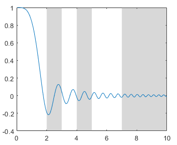
In apps, panning a plot containing ConstantLine or
ConstantRegion objects is smoother and the contents of the axes
update immediately as you pan. Previously, panning showed blank areas when you panned
outside of the original axes limits.
For example, on a Windows 10, Intel Xeon CPU W-2133 @ 3.60 GHz test system, if you run this code and then pan within the axes, the horizontal line and the gray vertical region update immediately as you pan.
function myapp
fig = uifigure;
ax = axes(fig);
x = -10:0.1:10;
y = sin(x);
plot(ax,x,y);
xlim(ax,[-6 6])
yline(ax,0)
xregion(ax,-3,3)
end
R2023a | R2023b |
|---|---|
The plot shows blank areas during the panning interaction.
| The plot updates immediately during the panning interaction.
|
When a user resizes an app figure window for the first time, many apps reposition their
content significantly faster in R2023b than in R2023a. The improvement occurs when resizing
an app with one or more containers that have the AutoResizeChildren
property set to "on", which is the default value. The improvement is
more noticeable for apps with nested containers, such as apps with many tabs or tab
groups.
For example, this code creates an app that contains five top-level tabs, each of which contains five nested tabs. Each of the nested tabs contains 100 edit fields. When you run this app and resize it, the resize operation is about 30x faster in R2023b than in the previous release.
function myApp
f = uifigure;
f.Position = [100 100 700 500];

% Create five tabs in a tab group
tg = uitabgroup(f,"Position",[1 1 700 500]);
nTabs = 5;
for kTab = 1:nTabs
    tab = uitab(tg,"Title","Tab " + kTab);
    createTabContent(tab);
end

    function createTabContent(tab)
        % Create a nested tab group containing five tabs
        nestedTg = uitabgroup(tab,"Position",[10 10 650 450]);
        nNestedTabs = 5;
        for kNTab = 1:nNestedTabs
            nestedTab = uitab(nestedTg,"Title","Nested Tab "+ kNTab);
            % Add 100 edit fields to the tab
            createNestedTabContent(nestedTab);
        end
    end

    function createNestedTabContent(tab)
        % Add 100 edit fields to a tab
        hParent = 400;
        n = 10;
        w = 50;
        h = 22;
        for kRow = 1:n
            for kCol = 1:n
                uieditfield(tab,"Position",[(kCol-1)*(w+10)+10,hParent-kRow*(h+10),w,h]);
            end
        end
    end
end
R2023a | R2023b |
|---|---|
The app takes about 60 seconds to resize.
| The app takes about two seconds to resize.
|
The resize interactions were times on a Windows 10, Intel
Xeon Gold 6246R CPU @ 3.40 GHz test system by running the myApp
function and measuring the time it takes for the figure window to resize.
Displaying images and 3-D plots in apps is significantly faster in MATLAB
Online. You might also experience similar improvements outside the context of an app
(by calling figure instead of uifigure).
For example, this code displays a scaled-up version of peppers.png
using the image command. The code is about 22x faster than in the
previous release.
function myapp
f = uifigure;
ax = axes(f);
smallimg = imread("peppers.png");
bigimg = uint8(zeros(3065,4089,3));
bigimg(:,:,1) = uint8(interp2(double(smallimg(:,:,1)),3));
bigimg(:,:,2) = uint8(interp2(double(smallimg(:,:,2)),3));
bigimg(:,:,3) = uint8(interp2(double(smallimg(:,:,3)),3));

tic
image(ax,bigimg)
drawnow
toc
end
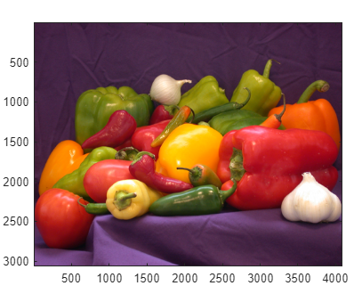
The approximate execution times are:
R2023a: 138.5 s
R2023b: 6.4 s
The code was timed by calling the myapp function. Because MATLAB
Online is hosted, performance is independent of the computer hardware used to access
it.
Software Development Tools
In MATLAB Online, you can use the Source Control panel to see all active source control repositories, manage modified files, and perform source control operations.
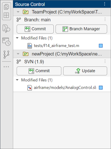
To open the Source Control panel, use the Open more panels button (![]() ) in the sidebar.
) in the sidebar.