Environment
MATLAB Desktop: Share files in MATLAB Drive from MATLAB
You can now share a file stored in MATLAB® Drive™ directly from MATLAB. When you share the file, MATLAB shares the folder that contains the file as well. Sharing files that are in the root MATLAB Drive folder is not supported.
To share a file, right-click the file in the Files panel, select Share, and then select from the available options. To manage permissions, select Invite Members and then add members with read or edit permissions to your file. To share your file with others through a link, select Create Link.
You also can now manage an already shared folder from inside that shared folder. To manage an existing shared folder, right-click any subfolder or white space inside the shared folder, select Share, and then select from the available options.
For more information, see Share Files Using MATLAB Drive.
Java Runtime: Install your own version of Java
MATLAB provides two-way integration with the Java® programming language and supports specific OpenJDK® long-term support (LTS) releases across all platforms. After installing MATLAB, you can install OpenJDK using the Add-On Explorer:
On the MATLAB Home tab, in the Environment section, click Add-Ons.
In the Add-On Explorer, search for
OpenJDK.Install the MATLAB Support for OpenJDK add-on.
In the MATLAB Command Window, clear the current JRE™ so that MATLAB uses the installed OpenJDK add-on.
jenv -clear
Alternatively, you can download and install any compatible OpenJDK distribution from https://adoptium.net/. For information about supported versions, see Versions of
OpenJDK Compatible with MATLAB by Release.
In a future release, MATLAB will no longer include Oracle® Java as part of its installation. For additional details, see Java Runtime will no longer be installed by default in a future release.
Live Editor Text: Create multilevel lists
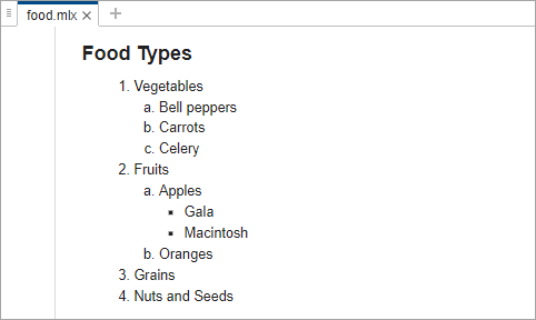
You can create multilevel bulleted or numbered lists in live scripts or functions. To create a multilevel list, with your cursor in a text line, go to the Live Editor tab and in the Text section, click the Bulleted list or Numbered list button. Then, press the Tab key to indent a numbered or bulleted item.
To decrease the indentation, press Shift+Tab. To change a sublist to a different list type, use the Bulleted list and Numbered list buttons.
For more information, see Format Text in the Live Editor.
Live Editor Text: Create multilevel lists
MATLAB Desktop: Access recent files and online training using MATLAB Home page
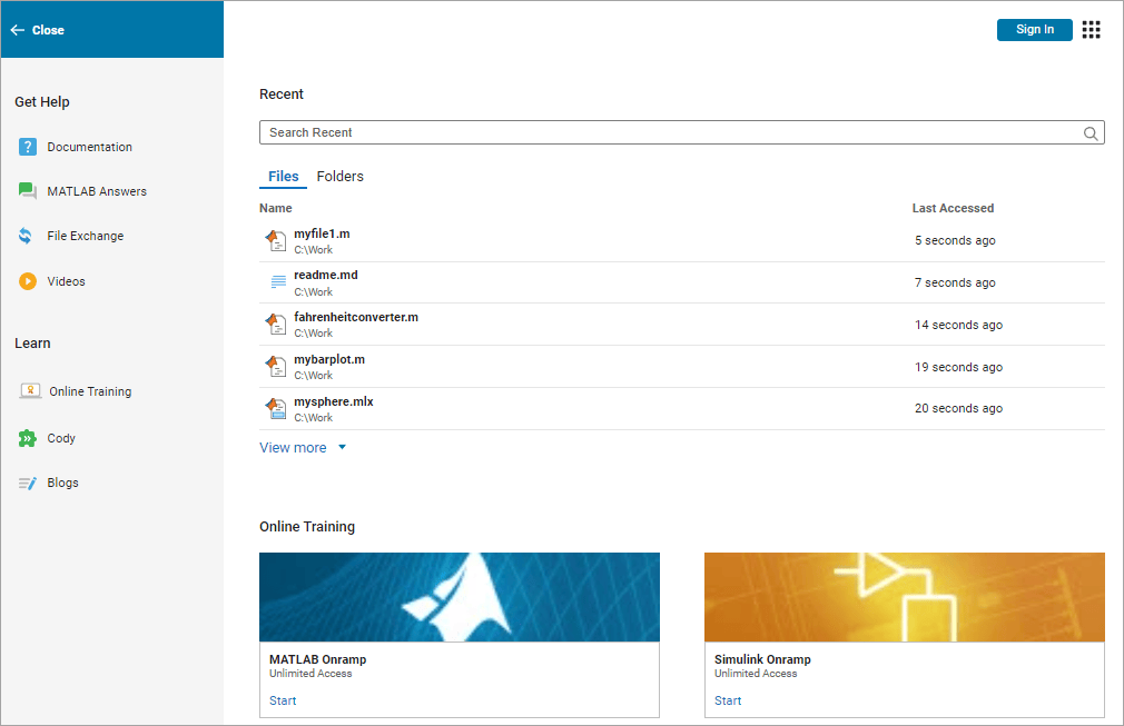
The new MATLAB Home page gives you quick access to your recent files, online training, and
other resources. To open the MATLAB Home page, in MATLAB, click the MATLAB Home button  to the left of the Home tab.
MATLAB Desktop: Access recent files and online training using MATLAB Home page
Live Editor Controls: Run custom code on button click
You can specify code to run when a button control is clicked in a live script. To
specify the code to run, right-click the button control in the live script and select
Configure Control. Then, in the
Execution section, set the Run option to
User-defined code and enter the code to run. When the button
is clicked, the specified code runs in the Command Window.
For more information, see Add Interactive Controls to a Live Script.
Live Editor Controls: Populate slider and spinner values using additional variable types
You can now populate the minimum, maximum, step, and default values for a slider or
spinner using values stored in a variable of any numeric type. Previously, only variables
of type double were supported.
For more information, see Link Variables to Controls.
Live Editor Tasks: Manage custom Live Editor tasks from the task gallery
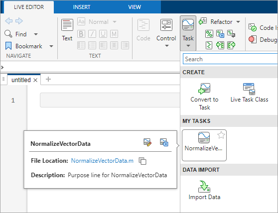
Manage a custom Live Editor task from the task gallery, including configuring task metadata, opening the task class definition file, and removing the task from the task gallery and from code suggestions. To view these options, hover over the Live Editor task icon in the task gallery.
Live Editor Tasks: Manage custom Live Editor tasks from the task gallery
Editor Spell Checker: Check spelling in MATLAB code and Markdown files by default
Spell checking is now on by default in the Editor and Live Editor. If a file contains many unrecognized words, such as when not written in US English, MATLAB automatically turns spell checking off for that file. In addition, spell checking is now supported in Markdown files.
To turn spell checking off by default, on the Home tab, in the
Environment section, click
Settings. Select MATLAB > Editor/Debugger > Spelling and set Check spelling to
Off. To change what text to spell check, in the Where
to check spelling section, select or clear the available options.
For more information, see Editor/Debugger Spelling Settings.
Editor Files: Change the default end-of-line sequence for new files
By default, the end-of-line sequence for new files on Windows® is the carriage return and line feed characters (\r\n). On
Linux® and macOS, the default end-of-line sequence for new files is the line feed character
(\n).
To change the default end-of-line sequence, go to the Home tab, and in the Environment section, click Settings. Select MATLAB > Editor/Debugger, and then select an option for Default end of line sequence.
For more information, see General Settings for the Editor/Debugger.
Editor Comments: Enhanced support for wrapping comments containing non-ASCII characters
The Editor and Live Editor now wrap comments containing non-ASCII characters, including emojis and CJK (Chinese, Japanese, and Korean) characters, more accurately and intuitively. Wrapped comments maintain proper alignment and readability, regardless of character width or encoding.
Comparison Tool: Compare folders and ZIP files using improved interface
Compare folders and ZIP files using an improved interface. Improvements include quick filters and new support for printable reports. For more information, see Compare Folders and ZIP Files.
Comparison Tool: Save comparison reports as PDF/A files
You can now save comparison reports as PDF/A files interactively and programmatically.
PDF/A comparison reports are not supported on Linux. For more information, see Compare Files and Folders and Merge Files and visdiff.
Cloud Storage in MATLAB: Connect to both your OneDrive Personal and OneDrive for Business accounts, including on macOS
MATLAB can now connect to both your OneDrive™ Personal and OneDrive for Business accounts at the same time.
In addition, if you have OneDrive set up on your macOS system, MATLAB now uses the OneDrive sync app to automatically connect to your OneDrive account.
For more information, see Use MATLAB to Access Files in Your Microsoft OneDrive.
Functionality being removed or changed
Java Runtime will no longer be installed by default in a future release
Behavior change in future release
Currently, MATLAB installations on Windows and Linux platforms include Oracle Java. However, in a future release, MATLAB will no longer include Oracle Java as part of its installation. Instead, you will have to download and install the MATLAB Support for OpenJDK add-on or any compatible OpenJDK distribution after installing MATLAB. MATLAB will continue to support OpenJDK on all platforms. For information about supported versions, see Versions of OpenJDK Compatible with MATLAB by Release.
For information about future changes to the jenv and
matlab_jenv functions, see Call Java from MATLAB: Configure JRE for the MATLAB Support for OpenJDK add-on.
Add-On Manager no longer supports updating add-ons
Behavior change
The Add-On Manager no longer supports updating an installed add-on. To update an add-on, use the Add-Ons panel instead. For more information, see Manage Add-Ons.
Command Window, Editor, Live Editor, and App Designer suggestions settings have moved
Behavior change
The suggestions settings for the Command Window, Editor, Live Editor, and App Designer have moved to the new MATLAB Suggestions Settings page in the Settings window. Previously, these settings were located on the MATLAB Command Window Suggestions Settings and MATLAB Editor/Debugger Suggestions and Autocompletions Settings pages. For more information, see Modify Suggestions Settings.
matlab.commandwindow.suggestions and
matlab.editor.suggestions settings have been removed
Errors
The matlab.commandwindow.suggestions and
matlab.editor.suggestions settings have been removed. Use the
matlab.suggestions settings instead. The behavior of the settings remains
the same.
This table shows how to update your code to use the
matlab.suggestions settings instead of the
matlab.commandwindow.suggestions and
matlab.editor.suggestions settings.
| Removed Setting (Errors) | New Setting |
|---|---|
matlab.commandwindow.suggestions.ShowAutomatically
| matlab.suggestions.commandwindow.ShowAutomatically
|
matlab.commandwindow.suggestions.ShowOnTab | matlab.suggestions.commandwindow.ShowOnTab |
matlab.commandwindow.suggestions.AcceptOnRightArrow
| matlab.suggestions.AcceptOnRightArrow |
matlab.commandwindow.suggestions.TabAcceptsOnOneSuggestion
| matlab.suggestions.commandwindow.TabAcceptsOnOneSuggestion
|
matlab.editor.suggestions.ShowAutomatically | matlab.suggestions.editor.ShowAutomatically |
matlab.editor.suggestions.ShowOnTab | matlab.suggestions.editor.ShowOnTab |
matlab.editor.suggestions.AcceptOnRightArrow | matlab.suggestions.AcceptOnRightArrow |
matlab.editor.suggestions.TabAcceptsOnOneSuggestion
| matlab.suggestions.editor.TabAcceptsOnOneSuggestion
|
matlab.editor.suggestions.ShowTips | matlab.suggestions.ShowTips |
info, helpdesk,
helpbrowser, support, and
whatsnew functions have been removed
Errors
The info, helpdesk,
helpbrowser, support, and
whatsnew functions have been removed.
To open the documentation, use the
docfunction.To get information about your MATLAB version, use the
versionfunction.To get help, see Contact Technical Support.
Language and Programming
Function Introspection: Get information about function signatures and argument validation
You can programmatically get information about function signatures and arguments using
the function metadata interface. Function metadata includes information about the input and
output arguments of a function. To access this information, use metafunction
to create a matlab.metadata.Function instance. The properties of this class provide details
about the input and output arguments and any validation applied to the arguments. You can
access details about class and size validation as well as validation functions and their
arguments.
metafunction also works for class methods. When you call
metafunction on a method, the function returns a matlab.metadata.Method instance. The properties of
matlab.metadata.Method use classes from the function metadata interface
to provide information about method input and output arguments.
matlab.metadata.Method Class: Get more information about method input
and output arguments using introspection
The matlab.metadata.Method class has a new
Signature property, which provides more detailed information than
the existing InputNames and OutputNames
properties. The Signature property is an instance of matlab.metadata.CallSignature, which provides not just the names of input and
output arguments, but also information about argument validation and default values.
MATLAB will continue to recognize the InputNames and
OutputNames properties.
Validation Functions: Use mustBeSorted to validate that array
elements are sorted
Use the mustBeSorted
function to validate that all elements of an input array are sorted. This function extends
the existing validation functionality for function argument and property validation
checks.
For more information, see Function Argument Validation and Property Validation Functions.
Validation Functions: Compare arrays with compatible sizes
These validation functions now support implicit expansion when comparing two inputs with compatible array sizes, similar to the implicit expansion behavior in arithmetic operations:
For example, the compareValues function restricts input argument
values using the mustBeGreaterThan validation
function.
function obj = compareValues(startValue,endValue)
    arguments
        startValue
        endValue {mustBeGreaterThan(endValue,startValue)}
    end
end
compareValues function now accepts inputs with
compatible array
sizes.compareValues([-2; -1],[3 2 1])
In previous releases, calling compareValues on 2-by-1 and 1-by-3
input arrays returned this
error:
Error using compareValues (line 4)
Second input to function 'mustBeGreaterThan' must be a scalar.
Metadata: Get information about functions, classes, and inner namespaces contained in a namespace
You can get information about the contents of a namespace by using these functions:
namespaceFunctions— Returns an array ofmatlab.metadata.Functionobjects that represent the functions defined in the specified namespace.namespaceClasses— Returns an array ofmatlab.metadata.Classobjects that represent the classes defined in the specified namespace.innerNamespaces— Returns a string array of inner namespace names in the specified namespace.
The methods matlab.metadata.Namespace.fromName and
matlab.metadata.Namespace.getAllNamespaces are no longer
recommended.
Properties containing classes that use custom indexing can use the
WeakHandle attribute
Properties that contain classes that use custom indexing can now be defined using the
WeakHandle attribute. This includes classes that inherit from
matlab.mixin.indexing.RedefinesParen or that override
subsref or subsasgn. For more information, see Property Attributes.
Dynamic Properties: GetAccess and SetAccess
attributes of dynamic properties can be metaclass objects
The GetAccess and SetAccess attributes of
dynamic properties can be a metaclass object or cell array of metaclass objects. For more
information, see Set Dynamic Property Attributes.
MATLAB Vault: Import secrets and update secret names and metadata
You can manage secrets in your MATLAB vault using these new functions:
importSecrets– Import secrets from ENV files into your MATLAB vault.renameSecret– Rename secrets in your MATLAB vault.removeSecretMetadata– Remove the metadata of individual secrets from your MATLAB vault.
Functionality being removed or changed
Change in precedence for functions and classes in @-folders with the same name
Behavior change
When a class defined in a class folder (@-folder) has the same name as a function, MATLAB now gives precedence to the item found earlier on the path. In previous releases, classes in class folders took precedence, regardless of path order.
Property get and set methods retrieved from introspection
Warns
You can currently invoke class property get and set methods using the handle returned
from a matlab.metadata.Property instance. In a future release, you will
not be able to do so for non-dynamic properties.
For example, obj is an instance of ClassA, which
defines Prop1 and a get method. If you retrieve the function handle
for the get method of Prop1 using introspection and invoke it,
MATLAB currently displays a warning.
mc = ?ClassA;
getProp1 = mc.PropertyList(1).GetMethod;
getProp1(obj)
Warning: Invoking set or get method 'ClassA.get.Prop1'. Invoking a
set or get method function_handle obtained from a
matlab.metadata.Property instance will error in a future release.

ans =

     value
Specialized operators of matlab.mixin.Scalar are now hidden
Behavior change
For the matlab.mixin.Scalar class, the specialized operators end,
isempty, isscalar, length,
ndims, numel, and size are now
hidden. The behavior of the operators remains the same.
Some validation functions no longer restrict inputs to be real, numeric, or logical
Behavior change
The following function argument and property validation functions no longer restrict
inputs to be real, numeric, or logical. The validation functions no longer call the
isreal, isnumeric, and
islogical functions to validate their inputs:
Similarly, mustBeNonzero no longer calls
isnumeric and islogical.
As a result, the validation functions accept any input types supported by the
underlying comparison operators and functions they use. For instance,
mustBeGreaterThan now accepts any data type supported by the
gt (or >) function,
such as character vectors, strings, and date and time types.
For example, the compareValues function restricts input argument
values using the mustBeGreaterThan validation
function.
function obj = compareValues(startValue,endValue)
    arguments
        startValue
        endValue {mustBeGreaterThan(endValue,startValue)}
    end
end
compareValues function now accepts data of
type datetime as
input.A = datetime("yesterday"); B = datetime("today"); compareValues(A,B)
In previous releases, calling compareValues with
datetime inputs returned this
error:
Error using compareValues (line 4)
Inputs to function 'mustBeGreaterThan' must be numeric or logical.
To preserve the behavior of previous releases, explicitly use mustBeReal and mustBeNumericOrLogical in your validation
checks. For example, this code preserves the previous behavior of
mustBeGreaterThan in the compareValues function
definition.
function obj = compareValues(startValue,endValue)
    arguments
        startValue {mustBeReal,mustBeNumericOrLogical}
        endValue {mustBeReal,mustBeNumericOrLogical, ...
                  mustBeGreaterThan(endValue,startValue)}
    end
end
mustBeNonzero, you can add
mustBeNumericOrLogical to retain the previous input
restrictions.Implicit default value for properties whose class is an enumeration based on numeric or logical values
Behavior change
When assigning a default value to a property whose class is an enumeration based on
numeric or logical values, MATLAB now uses the first listed enumeration member as the default, regardless of
its underlying numeric value. For example, in the MyContainer class, the
default value of Prop1 is MyFirst.
classdef MyContainer
    properties
        Prop1 (1,1) MyEnum
    end
end
classdef MyEnum < uint8
    enumeration
        MyFirst (1)
        MyZero (0)
        MySecond (2)
        MyThird (3)
    end
end
In previous releases, when MATLAB assigns a default value in a case like this, it uses the zero-based
enumeration member regardless of the order the enumerations are defined in. For example,
before R2026a, the default value of Prop1 in the class
MyContainer is MyZero.
Enumerations derived from numeric superclasses no longer support sparse underlying values
Behavior change
Enumerations derived from numeric superclasses can no longer have sparse underlying values.
Text-to-enumeration conversion produces error if more than one case-insensitive match exists
Behavior change
When converting text to an enumeration member, MATLAB errors if the text is a case-insensitive match for more than one
enumeration member. For example, calling Colors("reD") with this
enumeration errors because "reD" is a case-insensitive match for both
Colors.Red and
Colors.red.
classdef Colors
   enumeration
      Red
      Green
      red
   end
end
Defining classes: Using schema.m is not supported
Behavior change
Defining classes using schema.m files is not supported. Replace
existing schema-based classes with classes defined using the classdef keyword.
Defining classes: Using function syntax to define classes will
not be supported in a future release
Still runs
Support for defining classes using function syntax will be removed
in a future release. With appropriate code changes, replace existing function-based
classes with classes defined using the classdef keyword.
handle function returns
matlab.graphics.GraphicsPlaceholder arrays in some
circumstances
Behavior change
In some circumstances, calling handle as a function returns a
matlab.graphics.GraphicsPlaceholder array. For example, calling
handle([]) now returns an empty
matlab.graphics.GraphicsPlaceholder array.
MATLAB on Intel Performance Hybrid Architecture processors uses all physical cores by default
Behavior change
When you run MATLAB on Intel® processors that have performance hybrid architecture, the default maximum
number of computational threads is now equal to the number of all physical Performance-
and Efficient-cores. Previously, the default maximum was the number of physical
Performance-cores. For more information on how to control the maximum number of
computational threads, see maxNumCompThreads.
MATLAB Online: Path information no longer saved automatically
Behavior change
In MATLAB
Online™, changes to the search path are not saved automatically between MATLAB
Online sessions. To save changes to the search path, call savepath
with no input. Doing so saves the current search path into MATLAB Settings. At sign-in,
MATLAB Online automatically loads the search path stored in Settings.
Data Analysis
fillmissing Function, Clean Missing
Data Live Editor Task, and Data Cleaner App: Use mean,
median, or mode to fill missing data
You can fill missing data with the mean, median, or mode of the nonmissing values along the operating dimension.
For the
fillmissingfunction, specify the"mean","median", or"mode"fill method.For the Clean Missing Data task and the Clean Missing Data cleaning method in the Data Cleaner app, when the method for cleaning missing data is
Fill missing, select theMean,Median, orModefill method.
Join Tables Live Editor Task: Switch order of input tables
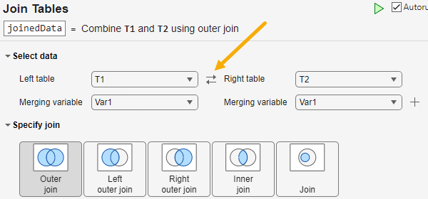
The Join Tables Live Editor task has a button for switching the order of the input tables. When you press it, the left table becomes the right table and the right table becomes the left table. The corresponding merging variables are switched along with the tables.
Join Tables Live Editor Task: Switch order of input tables
unique Function: Treat missing values as duplicates
For the unique function, you can treat repeated
instances of a missing value as duplicates. For example,
unique(A,TreatMissingAsDistinct=false) treats each instance of a
missing value in A as a duplicate value.
summary Function: Compute enumeration member counts
The summary function now computes the number of
occurrences of each member in an enumeration array. If you return a structure that contains
the summary, the Members and Counts fields contain
this information.
uminus and uplus Functions: Perform unary
minus and plus operations directly on tables and timetables
You can now call the uminus and uplus functions directly on tables and timetables without extracting their
data. All the variables in your tables and timetables must have data types that these
functions support. For more information, see Direct Calculations on Tables and Timetables and Rules for Table and Timetable Mathematics.
Functionality being removed or changed
mustBeInRange is not recommended
Still runs
The mustBeInRange function is not recommended. Use the mustBeBetween function instead. The mustBeBetween
function accepts more data types and uses a simpler way to specify the interval type,
using string values identical to those supported by the isbetween
function. However, there are no plans to remove
mustBeInRange.
This table shows some typical uses of mustBeInRange and how to
update your code to use mustBeBetween instead.
Not Recommended | Recommended |
|---|---|
mustBeInRange(A,0,100,"inclusive") |
mustBeBetween(A,0,100,"closed") |
mustBeInRange(A,0,1,"exclusive") |
mustBeBetween(A,0,1,"open") |
mustBeInRange(A,-5,5,"exclude-lower") |
mustBeBetween(A,-5,5,"openleft") |
Data Import and Export
JSON Files: Read and write JSON data as tables and timetables
Read and write JSON files using these functions:
readtableandreadtimetable— Read JSON data into MATLAB as a table or timetable. You can specify optional name-value arguments to control howreadtableandreadtimetabletreat JSON data.writetableandwritetimetable— Write a MATLAB table or timetable to a JSON file. You can specify optional name-value arguments to control howwritetableandwritetimetabletreat JSON data.
When reading JSON data, you can use the detectImportOptions function to detect aspects of the JSON file. When you
call detectImportOptions on a JSON file, it returns a JSONImportOptions object that you can use with readtable
or readtimetable to customize the import operation.
File Permissions: View and adjust permissions of multiple files using wildcards
You can view the permissions of multiple files by specifying their relative file paths
using a wildcard (*) with the filePermissions function.
You can then get or set individual permissions of multiple files by using the getPermissions and setPermissions functions, respectively.
FileDatastore Object: Read remote data from a local copy or its
source
You can choose whether to read remote data from a local copy or its original source
using the CreateLocalCopy name-value argument with fileDatastore. If you set CreateLocalCopy to
false, you avoid creating a local copy of your remote data to read
from. By default, CreateLocalCopy is true, and
fileDatastore downloads remote files before reading them.
delete Function: Remove multiple files by specifying a vector of
filenames
With the delete function, you can now remove
multiple files by specifying an input vector of filenames.
Comparison Tool: Compare and merge MAT files using improved interface
The Comparison Tool has an improved interface that lets you compare and merge MAT files more efficiently. Improvements include more intuitive merge interactions and new printable reports. For more information, see Compare and Merge MAT Files.
Merge Tool: Resolve conflicts in MAT files using Three-Way Merge tool
If conflicts occur in MAT files during a merge operation, you can now view and resolve the conflicts using the Three-Way Merge tool. For more information, see Resolve Conflicts in MAT Files.
MAT File Comparison: Automate comparison report generation for continuous integration (CI) workflows
You can now programmatically publish comparison reports for MAT files. Automate report
generation for continuous integration workflows using the visdiff function.
comparison = visdiff(matFile1,matFile2);
file = publish(comparison);
web(file)
FTP and SFTP: Remove subfolders, nonempty folders, and files using
rmdir
Remove subfolders, including nonempty folders, and files from FTP and SFTP servers using
the rmdir function with the
Recursive name-value argument. Specify Recursive
as true to recursively remove the contents of the specified folder. For
example:
f = ftp("ftp.example.com")
rmdir(f,"myfolder",Recursive=true)
xmlread Function: Specify XML processing engine for reading XML
file
When reading an XML file using the xmlread function, you can specify the XML processing engine as either the
MATLAB API for XML Processing (MAXP) or the Java API for XML Processing (JAXP). Specify the
XMLEngine name-value argument as "maxp" or
"jaxp", respectively.
xmlwrite Function: Specify MAXP DOM object for writing XML
file
When writing data to an XML file using the xmlwrite function, you can specify a MATLAB API for XML Processing (MAXP)
Document Object Model (DOM) node object as the DOMnode input argument.
Previously, the function accepted only a Java API for XML Processing (JAXP) DOM
object.
isfilePathInclusive Function: Determine if input is file in current
folder, specified location, or MATLAB path
To determine if an input is a file in the current folder, specified location, or
MATLAB path, use isfilePathInclusive.
Image Files: imfinfo now returns all EXIF tags associated with
HEIF and HEIC images
You can now use imfinfo to get information about all EXIF
tags associated with the HEIF or HEIC image files. Previously, imfinfo
could return only EXIF orientation tags associated with these images.
This functionality requires MATLAB Support for HEIF/HEIC Image Format, which is available only in the MATLAB desktop environment.
Parallel Processing: Use CFITSIO interface in thread-based environments
You can use the high-level and low-level functions from the CFITSIO interface in
thread-based environments, including MATLAB
backgroundPool.
For a list of high-level and low-level FITS functions, see FITS Files.
Comparison Tool: Compare schemas of HDF5, netCDF, and SOFA files
You can compare the schemas of HDF5, netCDF, and SOFA files by using the Comparison Tool.
The tool compares the schemas, but not the data, for these file types. Open the Comparison
Tool using the visdiff function.
Scientific File Format Libraries: NetCDF library upgraded to version 4.9.3
The netCDF library is upgraded to version 4.9.3.
Scientific File Format Libraries: CFITSIO library upgraded to version 4.5.0
The CFITSIO library is upgraded to version 4.5.0.
Scientific File Format Libraries: CDF library upgraded to version 3.9.1
The CDF library is upgraded to version 3.9.1.
VideoWriter Function: Support for code generation
The VideoWriter function now supports C/C++
code generation using MATLAB
Coder™ for MPEG-4 and AVI profiles.
Functionality being removed or changed
fileattrib function is not recommended
Still runs
The fileattrib function is not recommended.
View and edit file, folder, and symbolic link permissions using the filePermissions function
instead. However, there are no plans to remove fileattrib.
H5.open
and H5.close functions are not recommended and have no
effect
Behavior change
The H5.open and H5.close functions are not
recommended and have no effect. Previously, these functions could be used to open and
close the HDF5 library in MATLAB. You can still use type-specific functions to open and close HDF5 objects.
For example, use the H5F.open
and H5F.close
functions to open and close an HDF5 file.
disp displays partial content of tall arrays
Behavior change
Starting in R2026a, when you use the disp function to display the content of a tall array, MATLAB displays the top eight rows of data in the tall array. In previous
releases, MATLAB displays all the content of the tall array.
For example, this code creates a tall table. In R2025b, MATLAB gathers and displays all the content of the tall table. In R2026a, MATLAB displays only the top eight rows of the tall table.
tt = tall(table(randn(10,1),randn(10,1)));
disp(tt)
| Output in R2025b | Output in R2026a |
|---|---|
Evaluating tall expression using the Local MATLAB Session:
- Pass 1 of 1: Completed in 0.026 sec
Evaluation completed in 0.033 sec
      Var1        Var2
    ________    ________

    0.082831      -1.348
     -1.5485     -1.7543
      1.8632    -0.36381
     0.13403    -0.62709
      -1.546     0.44015
     0.43328     -1.5026
     0.10295    -0.20824
    -0.57035     -1.5051
     0.49306      1.8097
-0.70751 -0.1169 |
      Var1         Var2
    _________    ________

      0.87953     0.14766
      -1.4719      1.0809
     -0.27083    -0.05657
    -0.033141     0.17398
      0.53181      1.1838
      0.35187       0.927
      -1.1447     0.65327
      -1.8123     -0.8267
        :           :
: : |
To re-create the previous behavior, you can gather the tall array into memory and then display the content of the gathered array.
disp(gather(tt))
gather operation by
displaying the output of the tall array without using a semicolon. This will show the
top eight rows of data in the tall array.Mathematics
ode Object: Calculate Jacobians using automatic
differentiation
You can use the JacobianMethod property of an ode object to
specify whether the solver calculates the Jacobians for a given problem using finite
differences or automatic differentiation. By default, the Jacobians are calculated using
finite differences. The automatic differentiation method might be faster for large stiff
systems and more accurate for sensitivity analyses.
ode Object: Solve implicit ODEs using IDAS solver
You can now solve implicit ODEs using the IDAS solver by specifying the
Solver property of a fully implicit ode object as
"idas".
MATLAB Support Package for Quantum Computing: Parameterize circuits in local simulation (July 2026)
You can create parameterized rotation gates by specifying the rotation or phase angle as a parameterized expression using a string scalar, string vector, symbolic scalar, or symbolic vector in these creation functions:
Quantum circuits now have a Parameters property that lists the
parameters used by circuit gates. If a circuit has parameterized gates, you can specify
parameter values when calling the simulate, getMatrix, and observe functions on the circuit.
Functionality being removed or changed
Combining exponentiation operators with unary operators or logical negations without parentheses will not be supported in a future release
Still runs
When you specify a sequence of exponentiation operators combined with unary operators
or logical negations in the exponents, you will have to use parentheses to explicitly
specify the order of operations. Omitting parentheses in operations that include
^-, .^-, ^+,
.^+, ^~, or .^~ when chained
with other exponentiation operators will result in an error in a future release.
For example, the result of an operation such as y = 4^-3^-2
depends on the order in which exponentiation and negation are performed. For this
reason, use parentheses to explicitly specify the intended order of operations. For
example:
y = (4^(-3))^(-2)
y =
    4096
y = 4^(-(3^(-2)))
y =
    0.8572
y = 4^((-3)^(-2))
y =
    1.1665
conv function returns row vector for full convolution unless both
input vectors are column vectors
Behavior change
For the conv function, when you compute a full
convolution using w = conv(u,v) or w =
conv(u,v,"full"), the output w is a row vector unless
both input vectors u and v are column
vectors.
For example, if you convolve a row vector and a column vector, the output is a row vector.
u = [1 0 1];
v = [2; 7; 4];
w = conv(u,v)
w =
2 7 6 7 4u = [1; 0; 1]; v = [2; 7; 4]; w = conv(u,v)
w =
     2
     7
     6
     7
     4
In previous releases, when computing a full convolution, the conv
function returned either a row or column vector depending on the orientations and
lengths of u and v.
For example, in previous releases, conv returned the full
convolution of a 1-by-3 row vector and a 3-by-1 column vector as a 5-by-1 column
vector.
u = [1 0 1];
v = [2; 7; 4];
w = conv(u,v)
w =
     2
     7
     6
     7
4conv returned the full convolution of
a 1-by-3 row vector and a 2-by-1 column vector as a 1-by-4 row
vector.u = [1 0 1]; v = [2; 7]; w = conv(u,v)
w =
     2     7     2     7
There are no changes to the output of w = conv(u,v,"same") or
w = conv(u,v,"valid"), where the output still follows the
orientation of the first input vector u.
cast, double, single,
int8, int16, int32,
int64, uint8, uint16,
uint32, and uint64 functions preserve
complexity when converted complex input has zero imaginary part
Behavior change
The cast, double, single, int8, int16, int32, int64, uint8, uint16, uint32, and uint64 functions preserve complexity
when converting a complex input, even if the converted result has a zero imaginary
part.
For example, convert a complex number of type double to type
single. The output is a complex number of type
single with a zero imaginary
part.
a = complex(1,1e-48);
b = cast(a,"single")
b = single 1.0000 + 0.0000i
whos
  Name             Size            Bytes  Class     Attributes

  a                1x1                16  double    complex
  b                1x1                 8  single    complex
0.tf = isreal(b)
tf =

  logical
   0
For comparison, in previous releases, converting the same number returned a real
number of type
single.
a = complex(1,1e-48);
b = cast(a,"single")
b =
single
1whos
  Name             Size            Bytes  Class     Attributes

  a                1x1                16  double     complex
  b                1x1                 4  single
1
instead.tf = isreal(b)
tf =

  logical
   1
pow2 and log2 functions no longer accept
complex inputs when you specify two inputs or two outputs
Errors
The pow2 and log2 functions return an error if you specify complex inputs when using
the two-input or two-output syntax. These syntaxes no longer accept complex inputs. In
previous releases, the two-input syntax of pow2 and the two-output
syntax of log2 ignored the imaginary parts of complex inputs and
processed only the real parts.
To preserve the behavior of previous releases, use the real
function to extract the real parts of complex inputs, as shown in this table.
| Not Recommended (Errors) | Recommended |
|---|---|
X = 2 + 1i; E = 2i; Y = pow2(X,E); |
X = 2 + 1i; E = 2i; Y = pow2(real(X),real(E)); |
X = 2 - 1i; [F,E] = log2(X); |
X = 2 - 1i; [F,E] = log2(real(X)); |
pol2cart and sph2cart functions no longer
accept complex inputs
Errors
The pol2cart and sph2cart functions return an error for complex inputs. These functions no
longer accept complex inputs because their inverse functions, cart2pol and cart2sph, do not accept complex
inputs.
To preserve the behavior of previous releases for complex inputs, use the formulas that map polar, cylindrical, or spherical coordinates to Cartesian coordinates, as shown in this table.
| Not Recommended (Errors) | Recommended |
|---|---|
theta = 2i; rho = 1i; [x,y] = pol2cart(theta,rho); |
theta = 2i; rho = 1i; x = rho*cos(theta); y = rho*sin(theta); |
azimuth = 1i; elevation = 2i; r = 1; [x,y,z] = sph2cart(azimuth,elevation,r); |
azimuth = 1i; elevation = 2i; r = 1; x = r*cos(elevation)*cos(azimuth); y = r*cos(elevation)*sin(azimuth); z = r*sin(elevation); |
Graphics
Web Canvas: Create webpages with interactive graphics
Create HTML files containing interactive web canvases directly from your MATLAB plots and live scripts. A web canvas is an interactive plot element within an HTML page. Most visualizations in a web canvas support pan, zoom, and rotate interactions.
You can open an HTML file containing a web canvas using a web browser with an internet connection, share the file with others, or host it on a web server. No MATLAB license is required to view and interact with graphics in a web canvas. For more information, see Display Interactive Graphics on Webpages.
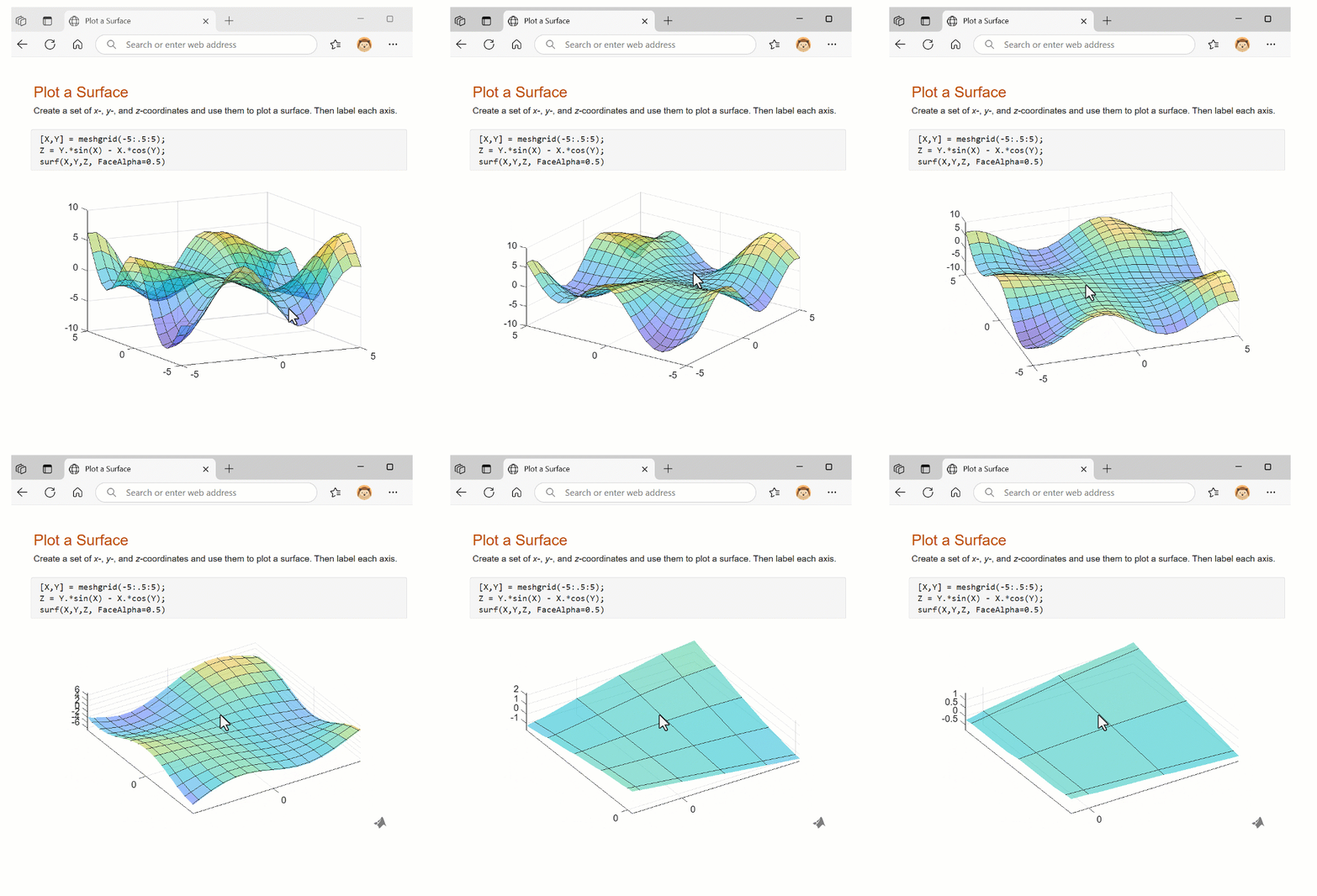
Web Canvas: Create webpages with interactive graphics
raincloudplot Function: Visualize grouped numeric data by using rain
cloud plots
To create rain cloud plots for grouped numeric data, use the raincloudplot
function. The upper half of each rain cloud plot displays a violin plot, and the lower half
displays a swarm chart. If you specify a matrix of input data,
raincloudplot creates a separate plot for each column in the
matrix. You can also specify a positional grouping variable to split your data into
groups.
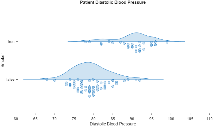
raincloudplot Function: Visualize grouped numeric data by using rain cloud plots
Plotting Table Data: Create plots by passing tables directly to plotting functions
These plotting functions now accept tables, timetables, and table variables as input
arguments: bar, barh, area, histogram, polarhistogram, geodensityplot, and binscatter.
In most cases, the axis labels and the legend (if present) automatically display the table
variable names.
Axes Toolbar: Interact with axes content using improved interface
The axes toolbar has an improved interface for interacting with axes content.
The toolbar appears persistently on axes. You can expand and collapse the toolbar by clicking a button. Previously, the toolbar appeared only when you hovered your mouse over the axes.
The appearance of the toolbar automatically matches the theme of the figure.
The toolbar is keyboard accessible and compatible with touchscreens and screen readers.
The toolbar supports SVG files for button icons and uses them by default. Previously, the only file types that the toolbar supported for icons were PNG, JPEG, and GIF. SVG icons allow for a sharper appearance than PNG and JPEG icons.
Additionally, the toolbar has a new property named Expanded.
Specify Expanded as "off" (the default) to collapse
the toolbar, and as "on" to expand the toolbar..
Axes Toolbar: Specify location of toolbar relative to axes
Specify the location of the axes toolbar relative to the axes by using the
ToolbarLocation property of the axes object. By default, MATLAB®
automatically selects the toolbar location based on the current view.
Axes Toolbar: Display or hide axes toolbar in standalone visualizations
Display or hide the axes toolbar in pie charts, donut charts, scatter histograms,
parallel plots, bubble clouds, and heatmap charts by setting the ToolbarVisible property of the chart. The axes toolbar is visible in these
charts by default, but you can hide it by setting the property to
"off".
Axes Toolbar: Specify tooltip text for toolbar drop-down menus
When you create a custom drop-down menu for the axes toolbar using a
ToolbarDropdown object, you can specify tooltip text for the menu
button by setting its Tooltip
property. The tooltip text appears when you hover the pointer over the button.
imresize Function: Apply padding that replicates border
pixels
The imresize
function now supports padding that replicates the pixel values at the border of the image.
To apply padding that replicates border pixel values, specify the new
Padding name-value argument as "replicate". By
default, or if you specify the Padding name-value argument as
"symmetric", the imresize function applies
symmetric padding.
Stability and Memory Usage: Create graphics with improved stability and memory usage
Scatter plots, surface plots, pseudocolor plots, and images have improved stability and memory usage. As a result, you can create more of these visualizations from large data sets than in the previous release without experiencing crashes or system resource issues.
Functionality being removed or changed
opengl function has been removed
Errors
The opengl function has been removed. To query the graphics
renderer, use the rendererinfo function instead.
In R2025a, MATLAB stopped using OpenGL® technology to render graphics, so you no longer need to set the renderer in your graphics workflows.
Links are preserved across multiple calls to the linkaxes
function
Behavior change
Calls to the linkaxes function preserve links
established by prior calls to the function. Previously, calls to the
linkaxes function canceled links established by prior calls to the
function.
For example, link the x-axes of ax1 and
ax2 and then link the y-axes of
ax1 and
ax3.
linkaxes([ax1 ax2],"x")
linkaxes([ax1 ax3],"y")
ax1 and ax2. In
previous releases, the second function call canceled the link between the
x-axes of ax1 and ax2.To preserve the previous behavior, you can explicitly cancel prior links before creating a
new link. For example, to cancel all links involving ax1 or
ax2, call linkaxes([ax1 ax2],"off").
PickableParts property of Axes objects is
"all" by default
Behavior change
Starting in R2026a, the default value for the PickableParts property
of Axes, UIAxes, PolarAxes, and GeographicAxes
objects is "all". Previously, the default value was
"visible".
Figure Copy settings use consistent default figure sizes on all systems
Behavior change
In the MATLAB Figure Copy Settings window, if you clear the Match on-screen size check box with no other changes, or if you make other changes and click Restore Defaults, the default size of the copied figure is consistently 1000-by-600 pixels regardless of the display resolution.
Previously, if you changed the settings in these ways, the default size of the copied figure depended on the resolution of the system display, which often resulted in inconsistent image sizes.
imshow function always sets
InitialMagnification to "fit" in the Live
Editor
Behavior change
When you use the imshow function in the Live Editor, the
default value of the InitialMagnification name-value argument is
now "fit". Previously, the default value was 100,
and titles might have appeared cropped.
You do not need to update your code. If you specify
InitialMagnification in a live script, the function ignores it
without error. However, image sizes might differ from previous releases.
Marginal histograms of scatterhistogram plots update after
interaction is complete
Behavior change
If you create a scatterhistogram plot and then pan or zoom in a way that affects the
shape of the marginal histograms, the histograms update after you lift your finger from
your device or mouse.
Previously, the marginal histograms updated as you performed the interaction (before lifting your finger).
ButtonDownFcn property of AxesToolbar,
ToolbarStateButton, ToolbarPushButton, and
ToolbarDropdown objects has been removed
Errors
The ButtonDownFcn property of AxesToolbar,
ToolbarStateButton, ToolbarPushButton, and
ToolbarDropdown objects has been removed. Previously, these objects
each had a ButtonDownFcn property, but the property had no
effect.
Children property of ToolbarStateButton and ToolbarPushButton objects has been removed
Errors
The Children property of ToolbarStateButton and ToolbarPushButton objects has been removed. Previously, these objects each had a Children property, but the property had no effect.
App Building
UI Components: Associate label with component
Associate a label with the UI component that it describes by using the
Label property of the component. Screen readers use the label text
to describe the component when an app user navigates through your app.
For more information, refer to the object page of the labeled UI component. For example,
see the Label property of the edit field component.
App Designer: Share app in MATLAB Drive from App Designer
You can share an app that you have stored in MATLAB Drive directly from App Designer.
With the app open in App Designer, on the Designer tab, in the Share section, select Share > MATLAB Drive. To manage permissions, select Invite Members and then add members with read or edit permissions to your app folder. To share your app with others through a link, select Create Link.
For more information, see Share App in MATLAB Drive.
App Designer: View code details in Code View using status bar
When you have an app open in Code View, you can view details about your app code in the status bar at the bottom of App Designer. For example, you can view how many times a highlighted variable appears in your code or the name of the function your cursor is in.
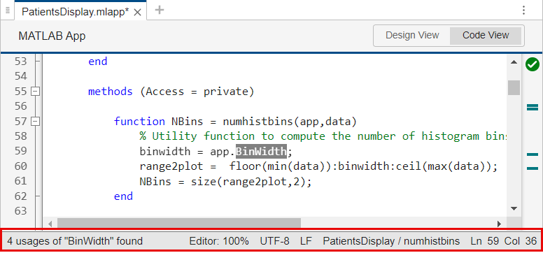
App Designer: View code details in Code View using status bar
App Designer: Update app layout and navigate code more easily
In Design View, when you move UI components on the canvas, you can constrain vertical or horizontal movement by holding Shift while you drag. For example, to move a button to the right without moving it up or down, hold Shift and then drag the button.
You can also reorder labeled components and other groups of components together. For example, to bring a component and its associated label to the front, select the component and its label, and then on the Canvas tab of the toolstrip, in the Arrange section, select Reorder > Bring to Front.
Finally, in Code View, in the Code Browser panel, when you select the name of a callback, function, or property, App Designer scrolls that element into view and highlights it in your code.
App Designer: Use custom keyboard shortcuts in Code View
Custom keyboard shortcuts that you specify for MATLAB now apply in App Designer Code View. You can use Emacs keyboard shortcuts or define your own custom shortcuts.
To change your keyboard shortcuts, in MATLAB, on the Home tab, in the Environment section, click Settings. Then, select Keyboard > Shortcuts. For more information, see Customize Keyboard Shortcuts.
App Designer: Remove Simulink dependency from app
For an app originally created as a blank app from the App Designer start page, App Designer now automatically removes all Simulink® dependencies whenever the app does not contain any Simulink functionality. For example, if you create a blank app, add a Simulink UI component, and then delete that Simulink UI component, App Designer removes the dependency on Simulink from that app.
Functionality being removed or changed
Interactions with app toolbar buttons have different keyboard shortcuts
Still runs
Interactions with buttons on an app toolbar have different keyboard shortcuts. The new shortcuts apply to push tool and toggle tool UI components and to buttons on an axes toolbar. These keyboard shortcuts are more consistent with keyboard shortcuts for other UI components in apps.
To move focus to a button on an app toolbar, use the Tab key. Once a button is in focus, use the arrow keys to navigate between different buttons on the toolbar.
In previous releases, the Tab key navigated between different buttons.
Performance
MATLAB Startup: Improved performance
MATLAB starts up faster in R2026a than in R2024b and previous releases. This improvement is most noticeable after the first startup and when starting MATLAB with multiple files open in the Editor.
For example, after the first startup, MATLAB R2026a starts up about 1.3x times faster than R2024b.
The approximate startup times are:
R2024b: 9.12 s
R2026a: 7.25 s
When starting with 15 code files previously open in the Editor, MATLAB R2026a starts about 1.4x times faster than R2024b.
The approximate startup times are:
R2024b: 11.24 s
R2026a: 8.22 s
Startup was timed on a Windows 11, Intel Xeon® 6-Core Processor @ 3.60 GHz test system by measuring the interval between launching MATLAB and the Command Window being ready to accept commands.
If your startup time is significantly slower than these approximate times, configuration issues or other factors might be affecting your MATLAB startup. For troubleshooting steps, see Resolve Slow Startup.
power Function: Improved performance when computing element-wise
powers with integer exponents
The power function (.^) shows
improved performance when computing element-wise powers with integer exponents. For
example, this code raises every element in a 5000-by-5000 array to the power of 3. The code
is about 3.8x faster than in the previous release.
function t = timingPower
x = rand(5000);
y = @() x.^3;
t = timeit(y);
end
The approximate execution times are:
R2025b: 0.80 s
R2026a: 0.21 s
The code was timed on a Windows 11, AMD EPYC™ 74F3 24-Core Processor @ 3.19 GHz test system by calling the
timingPower function.
This performance improvement arises from code changes that also result in slightly different round-off behavior in double precision, leading to more accurate results. For example, this code now returns a result that is more accurate to the 15th digit after the decimal point in long scientific notation.
format longE
y = 0.4543.^3
y =
9.376229100700000e-02Previously, the same code returned this result.
format longE
y = 0.4543.^3
y =
9.376229100699998e-02Note that MATLAB converts a decimal number input, like 0.4543, to the
nearest representable double-precision binary value, which might not be exactly equal to
the original decimal input. For this reason, although the .^ operator
is now more accurate in double precision, the result might differ from a calculation
performed using the exact representation of the operands.
log Function: Improved performance when computing natural logarithms
in double precision
The log function shows improved performance
when computing natural logarithms in double precision. For example, this code computes the
natural logarithms of 100,000,000 real numbers within the interval of 0 to 1000. The code
is about 2.8x faster than in the previous release.
function t = timingLog
x = rand(1,1e8)*1000;
y = @() log(x);
t = timeit(y);
end
The approximate execution times are:
R2025b: 0.79 s
R2026a: 0.28 s
The code was timed on a Windows 11, AMD EPYC 74F3 24-Core Processor @ 3.19 GHz test system by calling the
timingLog function.
This performance improvement arises from code changes that also result in slightly different round-off behavior in double precision, leading to more accurate results. For example, this code now returns a result that is more accurate to the 15th digit after the decimal point in long scientific notation.
format longE
Y = log(1.63340913276288)
Y =
4.906693231856701e-01Previously, the same code returned this result.
format longE
Y = log(1.63340913276288)
Y =
4.906693231856700e-01
Note that MATLAB converts a decimal number input, like 1.63340913276288,
to the nearest representable double-precision binary value, which might not be exactly
equal to the original decimal input. For this reason, although the
log function is now more accurate in double precision, the result
might differ from a calculation performed using the exact representation of the
input.
duration Data Type: Improved performance with
duration arrays
Operations on duration arrays show improved performance.
These operations include but are not limited to:
Arithmetic operations
Array creation
Array indexing
Concatenation
Reshaping
Sorting
For example, this code creates a duration scalar. The code is about
108x faster than in the previous release.
function timingTest
for i = 1:1e6
    d = duration(0,0,30);
end
end
The approximate execution times are:
R2025b: 12.93 s
R2026a: 0.12 s
As another example, this code assigns an element to a duration array.
The code is about 28x faster than in the previous release.
function timingTest
s = seconds(1:1e6);
for i = 1:1e6
    s(1) = 0;
end
end
The approximate execution times are:
R2025b: 0.57 s
R2026a: 0.02 s
The code was timed on a Windows 11, AMD EPYC 74F3 24-Core Processor @ 3.19 GHz test system using the
timeit function.
timeit(@timingTest)
filter Function: Improved performance for finite impulse response
(FIR) filters
The filter function shows improved performance
for FIR filters. FIR filters are characterized by a finite impulse response duration and a
rational transfer function in the z-domain that has only zeros and no
poles. The performance improvement is most noticeable when the transfer function has a
significant number of coefficients.
For example, this code filters an input signal of length 1,000,000 using a low-pass filter with 10,001 coefficients in the numerator of the transfer function. The code is about 2.3x faster than in the previous release.
function ts = timingFilter
t = 1:1000000;
x = sin(5e-5*t) + sin(10*t) + 0.1*rand(size(t));

N = 10000;
freq = 0.5;
k = -(N/2):(N/2);
h_ideal = sin(freq*pi*k)./(pi*k);
h_ideal(k==0) = freq;
w = 0.54 - 0.46*cos(2*pi*(0:N)/N);
b = h_ideal.*w;

y = @() filter(b,1,x);
ts = timeit(y);
end
The approximate execution times are:
R2025b: 0.28 s
R2026a: 0.12 s
The code was timed on a Windows 11, AMD EPYC 74F3 24-Core Processor @ 3.19 GHz test system by calling the
timingFilter function.
nufft and nufftn Functions: Improved performance
with nonuniform sample points and query points
The nufft and
nufftn
functions show improved performance when operating on nonuniformly spaced sample points and
query points. These functions achieve a significant performance increase by using more
efficient interpolation algorithms.
For example, this code computes the 1-D nonuniform discrete Fourier transform of a 10,000-by-1 array using 10,000 nonuniform sample points and 10,000 nonuniform query points. The code is about 330x faster than in the previous release.
function t = timing_nufft
n = 10000;
x = randn(n,1);
t = rand(n,1);
f = 10000*rand(n,1);

y = @() nufft(x,t,f);
t = timeit(y);
end
The approximate execution times are:
R2025b: 1.65 s
R2026a: 0.005 s
As another example, this code computes the 2-D nonuniform discrete Fourier transform along each dimension of a 100-by-100 array using 10,000-by-2 nonuniform sample points and 10,000-by-2 nonuniform query points. The code is about 123x faster than in the previous release.
function t = timing_nufftn
n = 100;
x = randn(n,n);
t = rand(n^2,2);
f = 100*rand(n^2,2);

y = @() nufftn(x,t,f);
t = timeit(y);
end
The approximate execution times are:
R2025b: 1.72 s
R2026a: 0.014 s
The code was timed on a Windows 11, AMD EPYC 74F3 24-Core Processor @ 3.19 GHz test system by calling the
timing_nufft and timing_nufftn functions.
kde Function: Improved performance of kernel density estimate
computations
The kde function
shows improved performance. The performance improvement depends on the size of the
univariate data set, the number of evaluation points, and the bandwidth for the kernel
smoothing function. For example, the kernel density estimate computation in this code is
about 15x faster than in the previous
release.
function timingTest
data = randn(1e5,1);
[f,xf,bw] = kde(data,NumPoints=1e4);
end
The approximate execution times are:
R2025b: 11 s
R2026a: 0.72 s
The code was timed on a Windows 11, Intel
Xeon CPU W-2133 @ 3.60 GHz test system using the timeit
function.
timeit(@timingTest)
join Function: Improved performance with tall tables when returning
two outputs
The join function
shows improved performance when the first input is a tall table and two output arguments
are returned. The second input argument can be either an in-memory table or the result of a
reduction operation on a tall table. The improvement is a result of reducing the number of
reads or passes through the tall table.
For example, this code joins a tall table and an in-memory table and gathers both the joined table and the index vector. The code is about 5.3x faster than in the previous release.
function t = timeJoinWithTwoOutputs
% Run tall code on the local MATLAB session
mapreducer(0)

% Create sample data
keysVar = (1:5e3)';
keysVarShuffled = randi(5e3,1e4,1);
x = randi(1e5,1e4,1);
y = randi(10,5e3,1);
z = randi(1e3,5e3,1,"single");
zz = randi(1e3,1e4,1,"single");

% Create tall table
t = table(x,keysVarShuffled,zz,VariableNames=["X","keys","ZZ"]);
tallTable = tall(t);

% Create in-memory table
inMemoryTable = table(y,z,keysVar,VariableNames=["Y","Z","keys"]);

% Measure time for join
    function joinWithTwoOutputs
        [C,idxb] = join(tallTable,inMemoryTable);
        gather(C,idxb);
    end
t = timeit(@joinWithTwoOutputs);
end
The approximate execution times are:
R2025b: 0.74 s
R2026a: 0.14 s
The code was timed on a Windows 11, Intel
Xeon Silver CPU 4310 @ 2.1 GHz test system by calling the
timeJoinWithTwoOutputs function.
innerjoin Function: Improved performance when joining tall and
in-memory tables
The innerjoin function shows improved
performance when the first input is a tall table. The second input argument can be either
an in-memory table or the result of a reduction operation on a tall table. The improvement
is a result of reducing the number of reads or passes through the tall table.
For example, this code performs an inner join of a tall table and an in-memory table and gathers the joined table into memory. The code is about 5.9x faster than in the previous release.
function t = timeInnerJoinWithTall
% Run tall code on the local MATLAB session
mapreducer(0);

% Create tall table
x = randi(1e3,1e4,1);
y = randi(1e3,1e4,1);
t = table((1:length(x))',x,y,VariableNames=["keys","Var1","Var2"]);
tallTable = tall(t);

% Create in-memory table
inMemoryTable = table(randperm(1e4,100)',x(1:100),y(1:100), ...
                VariableNames=["keys","Var3","Var4"]);

% Measure time for innerjoin
    function timeInnerJoin
        C = innerjoin(tallTable,inMemoryTable);
        gather(C);
    end
t = timeit(@timeInnerJoin);
end
The approximate execution times are:
R2025b: 1.58 s
R2026a: 0.27 s
The code was timed on a Windows 11, Intel
Xeon Silver CPU 4310 @ 2.1 GHz test system by calling the
timeInnerJoinWithTall function.
Data Grouping Functions: Improved performance for numeric or string grouping vector
These functions show improved performance when the grouping variable or vector type is
numeric or string:
When the grouping variable or vector is numeric, the improvement is most noticeable when the total number of elements and the number of elements per group are large.
For example, this code computes the group-wise mean for 12,500,000 elements split into 25 numeric groups. The code is about 9x faster than in the previous release.
function t = timingNumeric
numberOfGroups = 25;
elementsPerGroup = 5e5;
groups = repmat(1:numberOfGroups,1,elementsPerGroup)';
data = randn(numel(groups),1);
G = @() groupsummary(data,groups,"mean");
t = timeit(G);
end
The approximate execution times are:
R2025b: 1.35 s
R2026a: 0.15 s
When the grouping variable or vector type is string, the improvement
is most noticeable when the total number of elements is large and the number of elements
per group is small.
For example, this code computes the group-wise mean for 5,000,000 elements split into 50 string groups. The code is about 4.3x faster than in the previous release.
function t = timingString
numberOfGroups = 50;
elementsPerGroup = 1e5;
groups = repmat(string(1:numberOfGroups),1,elementsPerGroup)';
data = randn(numel(groups),1);
G = @() groupsummary(data,groups,"mean");
t = timeit(G);
end
The approximate execution times are:
R2025b: 1.03 s
R2026a: 0.24 s
The code was timed on a Windows 11, AMD EPYC 74F3 24-Core Processor @ 3.19 GHz test system by calling the
timingNumeric and timingString functions.
sort and sortrows Functions: Improved
performance for 8-bit and 16-bit integer data
The sort and sortrows functions show improved performance when sorting elements of type
int8, uint8, int16, or
uint16. The improvement is most noticeable when the number of
elements to sort is large.
For example, this code sorts a 100,000,000-element column vector of type
int8. The code is about 5.0x faster than in the previous
release.
function t = timingTest
A = randi(intmax("int8"),[1e8 1],"int8");
S = @() sort(A);
t = timeit(S);
end
The approximate execution times are:
R2025b: 1.06 s
R2026a: 0.21 s
The code was timed on a Windows 11, AMD EPYC 74F3 24-Core Processor @ 3.19 GHz test system by calling the
timingTest function.
readlines Function: Improved performance when reading lines of a
file as string arrays
The readlines
function shows improved performance when reading lines of data from a file as string
arrays. For example, this code creates a 48MB test file, reads the lines of data from the
file, and then deletes the file. The call to readlines is about 2.9x
faster than in the previous release.
function readlinesPerformance
%% Create the test file.
rng(1)
lines = 1e6;
lineLength = randi([30 70],[1 lines],"uint8");
fid = fopen("testfile.txt","W");
for ii = 1:numel(lineLength)
    data = randi([33 127],[1 lineLength(ii)],"uint8");
    fwrite(fid,[data 10],"uint8");
end
fclose(fid);

%% Timing test for readlines
f = @() readlines("testfile.txt");
t = timeit(f)

%% Delete test file.
delete testfile.txt;
end
The approximate execution times are:
R2025b: 0.85 s
R2026a: 0.29 s
The code was timed on a Windows 11, AMD EPYC 74F3 24-Core Processor @ 3.19 GHz test
system by calling the readlinesPerformance function.
mget Function: Improved performance when downloading files from SFTP
and FTP servers
The mget function shows improved performance
when downloading files from SFTP and FTP servers. For example, this code connects to an FTP
server, downloads a test file from the server into a local folder, and then deletes the
local folder and test file. The call to mget is about 1.6x faster than
in the previous release.
function mgetPerformance
f = ftp("ftp.ngdc.noaa.gov/geomag/wmm/");
m = @()mget(f,"wmm2015v2/shapefiles/2019_WMM2015v2_DI_shape_geographic.zip","localTestFolder");
t = timeit(m)
rmdir localTestFolder s
end
The approximate execution times are:
R2025b: 5.99 s
R2026a: 3.74 s
The code was timed on a Windows 11, AMD EPYC 74F3 24-Core Processor @ 3.19 GHz by
calling the mgetPerformance function.
ftp Function: Improved performance when connecting to
subfolders
The ftp function shows improved performance when
connecting to subfolders. For example, this code connects to a subfolder on an FTP server.
The call to ftp is about 2x faster than in the previous release.
function timingTest
ftp("ftp.ngdc.noaa.gov/pub/outgoing/mgg/nos/H13873/H13873/Raw/Positioning/FA_S220_EM712/2024-129/129_B");
end
The approximate execution times are:
R2025b: 0.94 s
R2026a: 0.48 s
The code was timed on a Windows 11, AMD EPYC 74F3 24-Core Processor @ 3.19 GHz using the
timeit function.
timeit(@timingTest)
Line Plot Interactions: Improved responsiveness for panning and zooming
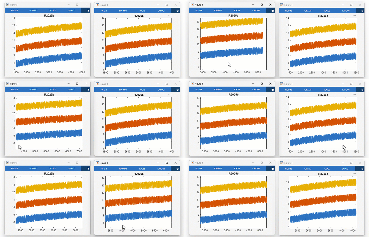
Line plots created using the plot function show improved responsiveness
for panning and zooming. If you plot approximately 2.5 million or more points and then pan
or zoom within the axes, the content that was previously outside the boundaries of the axes
comes into view more quickly in R2026a than in the previous release. Before R2026a, gaps in
the content appeared as you panned or zoomed.
For example, on a Windows 11, AMD EPYC 74F3 24-Core Processor @ 3.19 GHz test system that has an NVIDIA® A16-2B GPU with 2 GB RAM, if you run this code and then pan within the axes, the content updates immediately without any gaps.
x = 1:2500000;
y = [log(x') log(x')+2 log(x')+4] + rand(2500000,1);
plot(x,y)
xlim([1500 4500])
Quiver and Stem Plot Interactions: Improved responsiveness for panning and zooming
quiver and stem plots show improved responsiveness for panning and zooming. This
improvement is more noticeable when you plot approximately 25,000 or more points.
For example, on a Windows 11, AMD EPYC 74F3 24-Core Processor @ 3.19 GHz test system that has an NVIDIA A16-2B GPU with 2 GB RAM, if you run this code and then pan within the axes, the panning action is smoother and follows the cursor more closely in R2026a than in the previous release.
[x1,y1] = meshgrid(0:1:150, 0:1:300);
[x2,y2] = meshgrid(151:1:300, 0:1:300);
u1 = cos(x1);
v1 = sin(y1);
quiver(x1,y1,u1,v1,LineWidth=2)
hold on
u2 = cos(x2);
v2 = sin(y2);
quiver(x2,y2,u2,v2,LineWidth=2)
xlim([130 170])
ylim([130 170])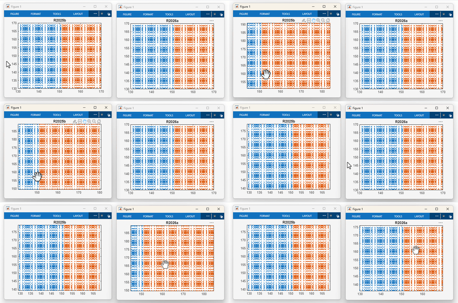
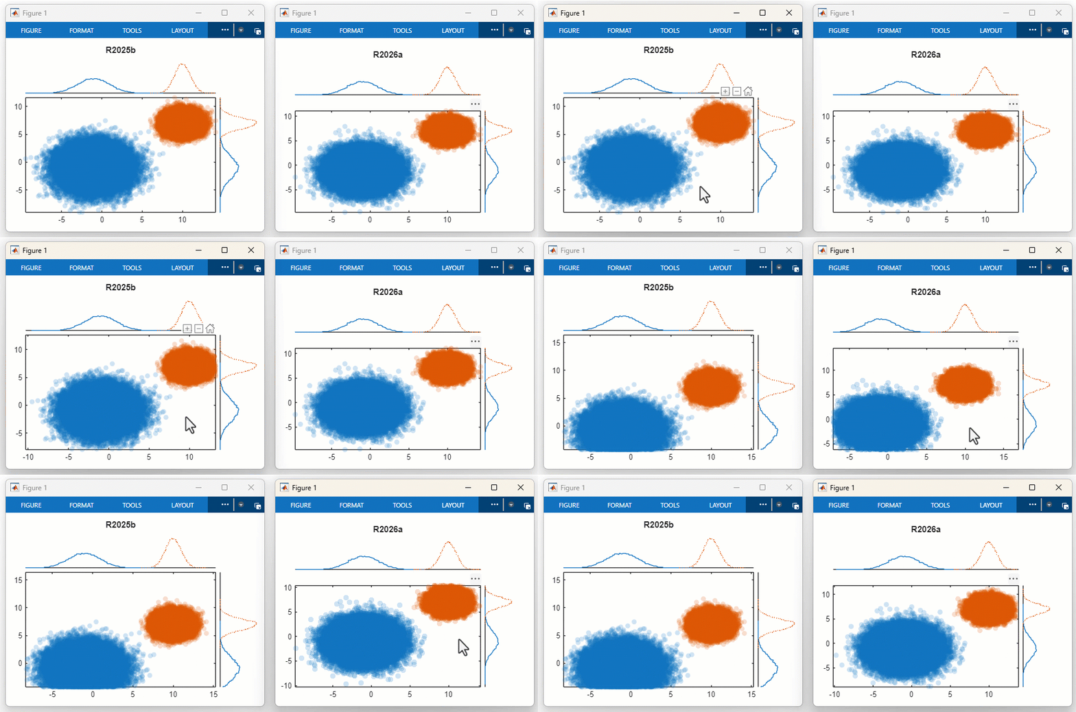
Scatter Histogram Interactions: Improved responsiveness for panning and zooming
Scatter histogram plots show improved responsiveness for panning and zooming. If you
plot a large number of points using the scatterhistogram function, the interaction is smoother and the visual
changes follow the cursor more closely.
For example, on a Windows 11, AMD EPYC 74F3 24-Core Processor @ 3.19 GHz test system that has an NVIDIA A16-2B GPU with 2 GB RAM, if you run this code and then pan within the plot, the panning action follows the cursor more closely in R2026a than in the previous release.
x1 = 2*randn(50000,1) - 1;
x2 = randn(50000,1) + 10;
y1 = 2*randn(50000,1) - 1;
y2 = randn(50000,1) + 7;
x = [x1; x2];
y = [y1; y2];
g = [ones(50000,1); ones(50000,1)*2];
scatterhistogram(x,y,GroupData=g,MarkerAlpha=0.2)
validatecolor and fliplightness Functions:
Improved performance for validating and flipping colors
The validatecolor
function shows improved performance, and this improvement positively impacts the
performance of the fliplightness
function.
For example, validate 125,000 colors. The call to validatecolor is
about 81x faster than in the previous release.
function t = timingTest
colors = rand(125000,3);
f = @() validatecolor(colors,"multiple");
t = timeit(f);
end
The approximate execution times are:
R2025b: 0.81 s
R2026a: 0.01 s
Flip the lightness of 125,000 colors. The call to fliplightness is
about 7.3x faster than in the previous release.
function t = timingTest
colors = rand(125000,3);
f = @() fliplightness(colors);
t = timeit(f);
end
The approximate execution times are:
R2025b: 0.88 s
R2026a: 0.12 s
The code was timed on a Windows 11, AMD EPYC 74F3 24-Core Processor @ 3.19 GHz test system that has an NVIDIA A16-2B GPU with 2 GB RAM by calling the timingTest
function.
Legends in Plots: Improved performance for legends with multiline labels and in plots with invisible objects
The legend function shows improved performance
when creating legends that have at least one multiline label or at least one entry that
represents an invisible object. The improvement becomes more noticeable as the number of
entries in the legend increases.
For example, create a line and 20 scatter plots. For each scatter plot, specify a legend
label that has two lines of text using the DisplayName name-value
argument. Then hide the line (p), and create a loop that displays a
legend, updates the figure, and deletes the legend 10 times. The minimum time for creating
a legend, updating the figure, and deleting the legend is about 1.9x faster than in the
previous release.
function mt = timingTest
x = 1:50;
y0 = 1:50;
p = plot(x,y0,DisplayName="Ideal");
hold on
% Create 20 plots
for k = 1:20
    y = 0.1*k*x + randn(1,50);
    scatter(x,y,DisplayName=["Trial" + string(k) + newline + "CohortA"])
end
hold off
p.Visible = "off";
% Create a legend 10 times
t = NaN(10,1);
for i = 1:10
    tic
    legend
    drawnow
    t(i) = toc;
    legend off
    drawnow
end
mt = min(t);
end
The approximate execution times are:
R2025b: 0.39 s
R2026a: 0.21 s
The code was timed on a Windows 11, AMD EPYC 74F3 24-Core Processor @ 3.19 GHz test system that has an NVIDIA A16-2B GPU with 2 GB RAM by calling the timingTest
function.
uiimage Function: Improved performance when resizing an app with
multiple images in a grid
When you resize an app figure window that contains multiple images created using the
uiimage
function and those images are in a grid layout manager, the app repositions its content
faster in R2026a than in R2025b. This improvement is more noticeable as the number of
images in the grid increases.
For example, this code creates an app that contains 400 images in a grid layout manager. When you run this app and resize it, the resize operation is about 3x faster than in the previous release.
function myApp
f = uifigure;
n = 20;
g = uigridlayout(f);
g.ColumnWidth = repmat(["1x"],1,n);
g.RowHeight = repmat(["1x"],1,n);

for k = 1:n
    for j = 1:n
        im = uiimage(g,ImageSource="peppers.png",ScaleMethod="fill");
    end
end
end
The approximate execution times are:
R2025b: 3 s
R2026a: 1 s
The resize operations were timed on a Windows 11, AMD EPYC 74F3 24-Core Processor @ 3.19 GHz test system by running the
myApp function and measuring the time it takes for the images in
the app to resize.
Test Browser App: Improved performance when adding and running tests
The Test Browser app shows improved performance when adding and running tests. The improvements result from reduced test browser overhead rather than changes to the underlying unit testing framework. Generally, the improvement becomes more noticeable as the number of tests increases. While add-time improvements are independent of test content, run-time improvements depend on the nature of the tests, including their complexity and outcomes.
For example, in a file named ExampleTest.m, create the
ExampleTest test class, which defines 1000 parameterized tests.
classdef ExampleTest < matlab.unittest.TestCase
    properties (TestParameter)
        value = num2cell(randi(10,1,1000))
    end

    methods (Test)
        function testValue(testCase,value)
            testCase.verifyNotEmpty(value)
        end
    end
end
When you click the Add tests button on the Test Browser toolbar and then select the specified test file, the test browser loads the tests about 5.5x faster than in the previous release. The approximate load times are:
R2025b: 13.1 s
R2026a: 2.4 s
When you click the Run current suite button on the toolbar, the test browser runs the added tests about 3.4x faster than in the previous release. The approximate run times are:
R2025b: 95.4 s
R2026a: 28.2 s
The test browser operations were timed on a Windows 11, Intel Xeon 6-Core Processor @ 3.60 GHz test system.
MATLAB Support Package for Quantum Computing: Improved performance when simulating quantum circuits
The simulate
function shows improved performance. For example, this code is about 32x faster than in the
previous update.
function timingTest
c = quantumCircuit(qftGate(1:20));
simulate(c);
end
The approximate execution times are:
R2025b (November 2025): 3.2 s
R2026a: 0.1 s
The code was timed on a Windows 11, Intel
Xeon CPU W-2133 @ 3.60 GHz test system using the timeit
function.
timeit(@timingTest)
Software Development
Project Checks: Detect case mismatch in project files, paths, and references
When you run project checks on Windows, the checks now detect case mismatch in project files, paths, and references.
For more information, see Run Project Checks and runChecks.
Project Filters: View files with status Not in project
In the Project panel, you can now filter files under the project root folder to view
only the files that have the status Not in project. For more
information, see Manage Project Files.
Project Settings: Reopen files from last time you opened project
When you close your project, MATLAB closes any open project files in the MATLAB Editor and reopens them the next time you open the project. You can disable this behavior by clearing the project setting Reopen MATLAB files from the last time you opened the project. For more information, see Configure Global MATLAB Projects Settings.
Project API: Create project object without opening the project
You can now create a project object for a project that is not loaded or open. For more
information, see matlab.project.Project.
Project API: Edit referenced project without opening it as top-level project
You can programmatically edit referenced projects without opening them as top-level projects.
For example, open a top-level project and create a project object for the referenced project. Then edit the referenced project without loading as a top-level project.
mainProj = openProject("MyTopLevelProject");
refProj = mainProject.ProjectReferences.Project;
addFile(refProj,"newFile.m");
openProject Function: Specify the project to load as a
matlab.project.Project object
The openProject
function now allows you to load a project by specifying a
matlab.project.Project object as the input.
Dependency Analyzer: Investigate file dependencies across projects in hierarchy
When you run a dependency analysis on a project that has referenced projects, you can investigate dependencies between files across projects in the project hierarchy using the Projects section in the Properties panel. For more information, see Examine File Dependencies Across Project Hierarchy.
Git Source Control: Switch branches from Source Control panel
You can switch Git™ branches directly by selecting a branch from the Branch drop-down list in the Source Control panel.
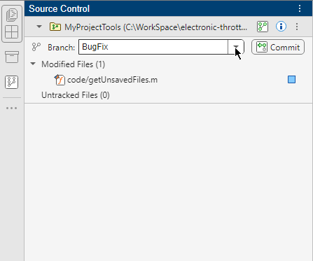
Git API: Create local branch that tracks remote branch and switch to it in one step
When you attempt to switch to a branch that exists only in a remote repository, the
switchBranch
function can now automatically create a local branch and set the upstream branch to the
remote tracking branch before switching to the new local branch.
repo = gitrepo;
branchDetails = switchBranch(repo,"remoteBranchName");StartPoint name-value
argument.switchBranch(repo,"remoteBranch",StartPoint="origin/remoteBranch");
Git API: Specify SSH passphrase when you interact with Git repository
If your SSH key is passphrase protected, you can now specify the SSH passphrase when you
programmatically interact with a Git repository using the gitclone, fetch,
pull, and
push
functions. For
example:
sshUrl = "git@github.com:user/examplerepo.git.";
gitclone(sshUrl,SSHUsername="user",SSHKeyPassphrase=getSecret("SSH_PASS"));
Git API: Clone single branch from Git repository
You can clone a single branch from a Git repository by specifying the new Branch and
SingleBranch name-value arguments with the gitclone function.
url = "https://github.com/domain/examplerepo";
gitclone(url,Branch="FeatureB",SingleBranch=true);
Source Control: Sign Git commits using SSH keys
Starting in R2026a, MATLAB supports signing Git commits using SSH keys. For more information, see Configure Git Settings.
mpmuninstall Function: Delete uninstalled packages from disk
When you uninstall packages and their dependencies using the mpmuninstall
function, you can specify the new Delete name-value argument as
true to delete the corresponding package files and folders
from disk.
Packages that are installed in-place are uninstalled but not deleted and must be removed from disk manually.
PackageIdentifier Object: Store package identifying
information
Use the matlab.mpm.PackageIdentifier object to store the identity information of a
specific package, including its name, version, and UUID. You can pass this object as an
input to any MATLAB Package Manager function that accepts a package specifier.
Build Automation: Run tasks in parallel
When you run a build in parallel, either programmatically using the buildtool
command or interactively from the MATLAB Toolstrip, the build tool executes tasks on the MATLAB client and workers in the current parallel pool (requires Parallel Computing Toolbox™). Previously, running a build in parallel affected only how
matlab.buildtool.tasks.TestTask instances ran.
The build tool considers task dependencies when scheduling a task to run in parallel. A task starts running in the parallel pool only after its dependencies have finished. For an example, see Run Tasks in Parallel.
Build Automation: View build summary in build output
When you run a build, the build output concludes with a build summary. The summary
includes the outcome and duration of the build, as well as an overview of task execution.
You can run a build either programmatically using the buildtool
command or the run method of
the matlab.buildtool.Plan class, or interactively from the MATLAB Toolstrip.
Build Automation: Control amount of build output interactively from Editor or MATLAB project
If your build file named buildfile.m is open in the MATLAB Editor or if your MATLAB project contains a build file named buildfile.m in its
root folder, then you can interactively control the amount of information displayed during
a build run from the MATLAB Toolstrip. For more information, see Run Build from Toolstrip.
Build Automation: Display test results in Test Browser
You can display the test results associated with matlab.buildtool.tasks.TestTask instances in the Test Browser app.
To use the test browser when running a build, first select the Use Test
Browser option in the Run Build section on the
MATLAB Toolstrip. Then, run your TestTask instances interactively
from the toolstrip or programmatically by specifying the -ui option of
the buildtool
command. For more information about the Use Test Browser option,
see Run Build from Toolstrip.
Build Automation: Specify threshold for informational messages when identifying code issues
When identifying code issues using a matlab.buildtool.tasks.CodeIssuesTask instance, you can specify the maximum
number of informational messages allowed for the task to pass by setting its
InfoThreshold property. If the number of informational messages
exceeds the specified threshold, then the task fails. You can set this property to perform
stricter checks on your code. By default, a CodeIssuesTask instance does not
fail on informational messages.
Unit Testing Framework: Add tests from currently open project to Test Browser
You can add the tests from the currently open MATLAB project to the Test Browser app.
To automatically add the tests defined in project files and folders with the
Test label, click the drop-down arrow to the right of the Add tests button
on the Test Browser toolbar and then select
Current Project. To also include the tests from referenced
projects, select Include Referenced Projects.
Unit Testing Framework: Add tests to Test Browser by dragging files and folders
You can add tests to the Test Browser app by dragging test files and folders from the Files or Project panel into the Test Browser panel. To include the tests in the subfolders of a dragged folder, first click the drop-down arrow to the right of the Add tests button on the Test Browser toolbar and select Include Subfolders.
Unit Testing Framework: Automatically open MATLAB project when running tests in project files and folders
If you run tests from test files and folders that belong to a MATLAB project, and that project is not already open, then the testing framework
automatically opens the project before running the tests and closes the project afterward.
This behavior occurs because the framework automatically includes a matlab.unittest.fixtures.ProjectFixture instance when creating a test suite
from test files and folders in a MATLAB project.
Unit Testing Framework: Test using parameterization properties that contain no data values
Parameterization properties can now contain an empty cell array or a scalar structure with no fields. When creating a test suite, the testing framework automatically excludes all the tests associated with parameterization properties that contain no data values. For an example, see Use External Parameters in Parameterized Test.
Unit Testing Framework: Generate test reports that have an improved appearance
Test reports generated using methods of the matlab.unittest.plugins.TestReportPlugin or matlab.unittest.TestResult class have an improved appearance. The improvements
include a redesigned cover page and support for viewing the contents in light or dark
theme.
The testing framework automatically selects colors that are visually appropriate for the theme. For example, text appears dark in light theme and light in dark theme. The theme of a report depends on where you view it:
A PDF or DOCX test report uses the theme of the application that renders it.
An HTML test report uses the theme of the MATLAB desktop. You can use the Toggle Theme switch at the top-left corner of the report to toggle between light and dark themes.
App Testing Framework: Programmatically interact with system dialog boxes
You can now use the chooseDialog
and dismissDialog
methods to programmatically interact with system dialog boxes created with the uigetdir, uigetfile, and uiputfile functions.
For example, create a test case for interactive testing.
testCase = matlab.uitest.TestCase.forInteractiveUse;
Dismiss the file selection dialog box that opens to the current folder.
dialogData = dismissDialog(testCase,"uigetfile",@uigetfile);Select the bin folder in the folder selection dialog box that opens
to the MATLAB root folder.
dialogData = chooseDialog(testCase,"uigetdir", ...
    @() uigetdir(matlabroot,"MATLAB Root Folder"), ...
    Folder=fullfile(matlabroot,"bin"));
App Testing Framework: Test Shift+click to select range of list box items
You can programmatically select a range of contiguous items in a list box by using the
choose method.
The choose method simulates the Shift+click action to
select contiguous list box items. For an example, see Select Multiple Items in List Box.
App Testing Framework: Interact with table row and column headers
You can now programmatically interact with table row and column headers by using the
press method.
The method allows you to click a table row or column header to select the corresponding row
or column, or click a sortable column header to sort the data in that column. For an
example, see Press Table Headers.
Mocking Framework: Create mocks for classes with abstract WeakHandle
properties
You can create mocks for classes that have properties with both the
Abstract and WeakHandle attributes. For an
example, see Create Mock for Class
with Abstract WeakHandle Property.
Functionality being removed or changed
mpmuninstall function returns an error for a package that is a
dependency
Behavior change
If you attempt to uninstall an installed package that is a dependency of another
package, the mpmuninstall function now returns an error.
Previously, if a package that was installed as a standalone package was also a
dependency of another installed package, then calling mpmuninstall
on that package did not uninstall the package but did change the
InstalledAsDependency property to true.
matlab.addons.toolbox.toolboxVersion function no longer
supports toolbox project files
Behavior change
When querying or modifying a toolbox version with the matlab.addons.toolbox.toolboxVersion function, you can now specify the
toolbox file as a MATLAB project file that contains a toolbox task. As part of this change, toolbox
project files (.prj) are no longer supported. To upgrade toolbox
project files to MATLAB project files with a toolbox task, open the toolbox project file as a
project in MATLAB. For more information, see Create and Share Toolboxes.
External Language Interfaces
External Languages Panel: View, create, and manage Python environments in MATLAB
You can use the new External Languages panel to manage external programming language environments in MATLAB. Starting in R2026a, you can add Python® environments, create virtual environments, switch between environments and execution modes, and manage libraries within Python environments.
To open the External Languages panel, click the Open more panels button
on any sidebar and select External
Languages. To manage Python environments using the External Languages panel, select the
Python option from the menu at the upper left. For more information,
see Manage Python Environments Using External Languages Panel.
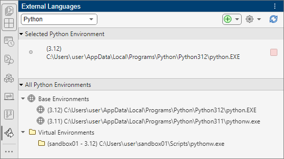
Call .NET from MATLAB: Unload .NET Core assembly from MATLAB
To unload a .NET Core assembly, set the Unloadable parameter to
true when you call NET.addAssembly and then call NET.unloadAssembly.
You cannot unload a .NET Framework assembly.
Call .NET from MATLAB: Compare two .NET objects for equality
Python: Support for CPython version 3.13
MATLAB now supports CPython version 3.13, in addition to existing support for versions 3.9, 3.10, 3.11, and 3.12. For supported version information, see Versions of Python Compatible with MATLAB Products by Release.
Call Python from MATLAB: Automatically convert MATLAB string array to Python list
When you pass data to a Python function, MATLAB automatically converts 1-by-N or N-by-1 MATLAB string arrays to Python lists.
For example, MATLAB converts the string array mlArr to a Python list.
mlArr = ["apple", "banana", "cherry"];
pyArrType = py.type(mlArr);
pystringarray Function: Convert MATLAB string arrays to NumPy string arrays
You can create a NumPy StringDType array from a multidimensional
MATLAB string array by using the pystringarray
function. The pystringarray function requires NumPy 2.0 or
greater.
Call Python from MATLAB: Compare two Python objects for equality
As of MATLAB R2024b, isequal and isequaln can compare two Python objects. You can use these functions to determine the equality of:
Two Python objects
A Python object and a MATLAB object that can be converted to a Python object
Two NumPy arrays
A NumPy array and a MATLAB array
In previous releases, isequal and isequaln do not
support the comparison of Python objects.
Call Java from MATLAB: Configure JRE for the MATLAB Support for OpenJDK add-on
The -clear option in the jenv and
matlab_jenv
functions removes the current JRE configuration for individual users or for each MATLAB installation for all users. After you install the MATLAB Support for
OpenJDK add-on from the Add-On Explorer, use the -clear option so
that MATLAB uses the add-on. For more information, see Configure Your System to Use Java.
If you call jenv or
matlab_jenv with the Java
version argument set to "factory", MATLAB sets the Java path to the version included with MATLAB. However, in a future release, MATLAB will no longer include Oracle
Java as part of its installation, and the argument value
"factory" will be removed. Likewise, the JavaEnvironment
Configuration property value "factory" will be
removed.
Call MATLAB from C++: Run MATLAB and your C++ application in the same process
You can run MATLAB in the same process as your C++ application. Call either matlab::engine::startMATLAB or matlab::engine::startMATLABAsync with mode set to
MATLABApplicationMode::IN_PROCESS. To run MATLAB in-process on Mac, you must also use matlab::engine::runMacLoopInProcess to start MATLAB on the main thread of the process and run your application logic on a
secondary thread.
Call MATLAB from C++: Support for matlab::data::Array data types in
matlab::engine::MATLABEngine functions feval and
fevalAsync
The matlab::engine::MATLABEngine member functions feval and fevalAsync support these
matlab::data::Array data types:
For more information, see the RhsArgs&&... rhsArgs entry in
the feval and fevalAsync Parameters
tables.
Web Services: Specify how to handle a basic authentication header
You can choose how a RESTful function treats a basic authentication header. By default,
a RESTful function first makes a request without credentials, receives a response that
indicates supported authentication methods, and then makes a second request using a
supported method. To specify that the RESTful function instead make the first request with
a Basic Authentication header field, create a weboptions object with the
BasicAuthenticationMethod name-value argument specified as
"preemptive". For more information, see weboptions.
MEX Functions: Build MEX functions from free-form Fortran source code
The mex command builds MEX functions from both
fixed-form and free-form Fortran source code. Free-form Fortran files typically use the
.F90 extension.
Compilers: Support for MinGW-w64 version 14.2 compiler on Windows, Microsoft Visual Studio 2026, and Intel oneAPI 2025 compiler
MATLAB supports the MinGW®-w64 version 14.2 compiler on Windows platforms. You can use this compiler to build C and C++ interfaces, MEX files, and standalone MATLAB engine and MAT-file applications. For installation instructions, see MATLAB Support for MinGW-w64 C/C++/Fortran Compiler.
MATLAB also supports Microsoft® Visual Studio® 2026.
As of R2025b, MATLAB supports these Intel compilers:
oneAPI 2025 compiler with Microsoft Visual Studio 2019 and 2022
oneAPI 2025 compiler for Fortran with Visual Studio 2019 and 2022
For continued support for building your applications, consider upgrading to a supported compiler. For an up-to-date list of supported compilers, see Supported and Compatible Compilers.
Perl 5.42.0: MATLAB support on Windows
As of R2025b, MATLAB for Windows includes an updated version of Perl, version 5.42.0.
If you use the perl command on Windows platforms, see https://www.perl.org/
for information about using this version of the Perl programming language.
Functionality being removed or changed
mex command will build MEX functions with the interleaved
complex API by default
Behavior change in future release
In a future release of MATLAB, the default api option
for the mex command will change to the interleaved complex API
(-R2018a). To prepare for the upcoming change, it is recommended that
you create new MEX files and update existing MEX files to use the interleaved complex API.
For more information, see MATLAB Support for Interleaved Complex API in MEX Functions.
If you want to continue using the separate complex API (-R2017b), then
explicitly specify the -R2017b option in your mex
command. For example, build MEX file myMexFile.c using the standard
complex API.
mex -R2017b myMexFile.c
For more information, see Upgrade MEX Files to Use Interleaved Complex API.
matlab.wsdl.createWSDLClient and
matlab.wsdl.setWSDLToolPath will be removed
Still runs
The matlab.wsdl.createWSDLClient and
matlab.wsdl.setWSDLToolPath functions
will be removed in a future release.
Use the MATLAB RESTful functions (webread and webwrite) or the MATLAB HTTP interface instead. For more information, see Call Web Services from MATLAB Using HTTP.
Hardware Support
Arduino Hardware: Support for Arduino Nano ESP32 and ESP32-S3-DevKitM-1 boards
You can now use MATLAB Support Package for Arduino® Hardware to communicate with the Arduino Nano ESP32 and ESP32-S3-DevKitM-1 boards over USB, Bluetooth®, and Wi-Fi® from an installed version of MATLAB. For more information on how to configure ESP32 boards, see Set Up and Configure ESP32 Hardware.
However, you cannot use the support package to connect these boards with an Adafruit® Motor Shield V2, motor carrier, CAN interface, or serial devices. The
function playTone and the name-value argument AnalogReferenceMode of the
arduino object in external mode do not
support these boards. For more information, see Supported Boards.
Arduino Hardware: Support for Raspberry Pi Pico and Pico W boards
You can now use MATLAB Support Package for Arduino Hardware to communicate with the Raspberry Pi® Pico boards over USB and the Pico W boards over USB and Wi-Fi in the MATLAB desktop environment. For more information, see Supported Boards.
Arduino Hardware: Support for Wi-Fi in MATLAB Online
You can now use MATLAB Support Package for Arduino Hardware to communicate with supported Arduino boards over Wi-Fi in MATLAB Online. For more information on the boards that support Wi-Fi, see Supported Arduino Boards, Workflows, and Platforms on MATLAB Online.
Arduino Hardware: Bluetooth support for Arduino Uno R4 Wi-Fi board
You can now use MATLAB Support Package for Arduino Hardware to communicate with the Arduino Uno R4 Wi-Fi board over Bluetooth. For more information, see Supported Boards.
Arduino Hardware: New example to estimate battery state of charge using deep learning
This release includes a new example that uses MATLAB Support Package for Arduino Hardware with Deep Learning Toolbox™. For more information, see Estimate Battery State of Charge Using Deep Learning with ESP32 Board.