Use Custom Constraints in Blending Process
This example shows how to design an MPC controller for a blending process using custom linear input/output constraints.
Blending Process
A continuous blending process combines three feeds in a well-mixed container to produce an output blend having the desired concentration of some constituents. The dimensionless governing equations are:
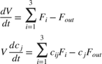
where
 is the volume of the mixture inventory in the container.
 is the volume flow rate for the input feed
  .
. is the volume flow rate for the blend exiting the container (the demand from downstream).
 is the concentration of constituent
  in the input feed .
 is the concentration of constituent in the output blend.
 is the time.
In this example, there are three feeds, = 1, 2 and 3 and two constituents, = 1 and 2.
The control objective is to maintain the following state variables at their setpoints:
the two constituent concentrations in the output blend (quality target)
the volume of the mixture inventory in the container (safety target)
The challenge is that the downstream demand, , and the concentration of the two constituents in the three input feeds, , can change from the nominal operating point.
The mixture inventory , the concentrations of the two constituents in the output blend  are measured, but the concentrations of the two constituents in the three input feeds are not measured.
At the nominal operating condition:
Input feed 1 has
 ,
,  and
and 
Input feed 2 has
 ,
,  and
and 
Input feed 3 has
 ,
,  and
and 
In addition, the plant only allows manipulation of the total feed flow rate entering the mixing chamber,  , and the individual flow rates of feeds 2,
  , and feed 3,
  . In other words, the flow rate of feed 1,
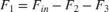
  , cannot be directly manipulated. However, is indirectly affected by the other three flow rates as follows:
Each input feed has limited availability imposed by the upstream process:

Define Linear Plant Model
The blending process is mildly nonlinear, given how the inventory volume enters the two concentration equations, however you can approximate it with a linear model at the nominal steady state. This approach is quite accurate unless the unmeasured concentrations of the two components in the three input feeds change. If the change is sufficiently large, the steady-state gains of the nonlinear process can change sign, and the closed-loop system can become unstable.
Specify the nominal flow rates for the three input streams and the output stream, or demand. At the nominal operating condition, the output flow rate is equal to the sum of the input flow rates.
Feed = [1.6,0.4,0];
F_out  = sum(Feed);
Define the nominal concentration of the two constituents in the input feeds, where cin(i,j) represents the concentration of constituent j in the input feed i. For example, the concentration of constituent 1 in input feed 2 is 0.2.
cin = [0.7 0.3;0.2 0.8;0.5 0.4];
Calculate the concentration of the two constituents in the output blend.
cout = Feed*cin/F_out;
The nominal volume of the mixture inventory is 2.
V = 2;
Create a state-space model with feed flows F1, F2, and F3 as inputs. The state variables of the linear model are the deviations from the nominal condition.
A = [0 0 0; 0 -F_out/V 0; 0 0 -F_out/V]; % 3 states are V, c1 and c2
Bu = [1 1 1; cin(:,1)'/V; cin(:,2)'/V]; % 3 inputs are F1, F2, F3
Since, as described above, the plant allows manipulation of the total input feed flow as well as the input feed flows 2 and 3 (with no direct control of the input feed 1), change the MV definition from [F1, F2, F3] to [F_in, F2, F3] using equation F1 = F_in - F2 - F3.
Bu = [Bu(:,1), Bu(:,2)-Bu(:,1), Bu(:,3)-Bu(:,1)]; % 3 inputs are F_in, F2, F3
Add the measured disturbance, the output blend demand, as 4th input.
Bv = [-1; -cout'/V];
B = [Bu Bv]; % 4 inputs are F_in, F2, F3, F_out
The outputs are just the state variables.
C = eye(3);
D = zeros(3,4);
Construct the structure that holds the linear plant model and its related information.
Model = ss(A,B,C,D);
Model.InputName = {'F_in','F_2','F_3','F_out'};
Model.InputGroup.MV = 1:3;
Model.InputGroup.MD = 4;
Model.OutputName = {'V','c_1','c_2'};
Create the MPC Controller
Specify the sample time, prediction horizon, and control horizon for the controller.
Ts = 0.1;
p = 10;
m = 3;
Create the controller.
mpcobj = mpc(Model,Ts,p,m);
-->"Weights.ManipulatedVariables" is empty. Assuming default 0.00000.
-->"Weights.ManipulatedVariablesRate" is empty. Assuming default 0.10000.
-->"Weights.OutputVariables" is empty. Assuming default 1.00000.
The outputs are the state variables, which are the inventory volume, y(1), and the concentrations of the two constituents in the output blend, y(2) and y(3). Specify nominal values for all outputs.
mpcobj.Model.Nominal.Y = [V cout(1) cout(2)];
Specify the nominal values for the manipulated variables, u(1), u(2) and u(3), and the measured disturbance, u(4).
mpcobj.Model.Nominal.U = [sum(Feed) Feed(2) Feed(3) F_out];
Specify output tuning weights. To emphasize controlling the concentration of the two constituents, use larger weights for the second and third outputs.
mpcobj.Weights.OV = [1 5 5];
Specify the hard bounds (physical limits) on input feeds 2 and 3, which are manipulated variables.
mpcobj.MV(2).Min = 0;
mpcobj.MV(2).Max = 1.6;
mpcobj.MV(3).Min = 0;
mpcobj.MV(3).Max = 1.6;
Specify Mixed Constraints
You cannot directly specify the lower and upper bounds of the flow rate for input feed 1, because it is not a manipulated variable. Instead, define the following linear inequality constraint and set it as a custom input/output constraint in the controller.

Specify this hard constraint in the form  .
.
E = [-1 1 1; 1 -1 -1];
F = [0 0 0; 0 0 0];
g = [0;1.6];
Set the custom constraints in the MPC controller.
setconstraint(mpcobj,E,F,g)
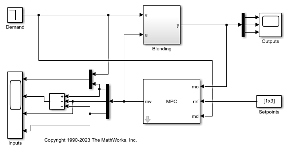
Simulate Model in Simulink
The Simulink® model contains a nonlinear model of the blending process and unmeasured disturbances in the concentrations of the two constituents in the three input feeds.
The Demand, , is modeled as a measured disturbance. The operator can vary the downstream demand value, and the signal goes to both the process and the controller.
The model simulates the following scenario:
At
 , the process is operating at the nominal operating point.
At
 , the demand decreases from
  to
to  .
.At
 , there is a change of the concentration both constituents in the input feed 1, from 0.7 and 0.3 to 0.6 and 0.4. Also, there is a change of concentration of constituent 1 in feed 3 from 0.5 to 0.4.
Open the Simulink model.
mdl = 'mpc_blendingprocess';
open_system(mdl)

% Simulate the model.
sim(mdl)

% Open the scope block windows.
open_system([mdl '/Inputs'])
open_system([mdl '/Outputs'])
-->Converting model to discrete time.
-->Integrator added as output disturbance model for measured output #2.
-->Integrator added as output disturbance model for measured output #3.
   Assuming no disturbance added to measured output #1.
-->"Model.Noise" is empty. Assuming white noise on each measured output.
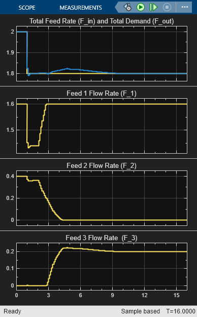
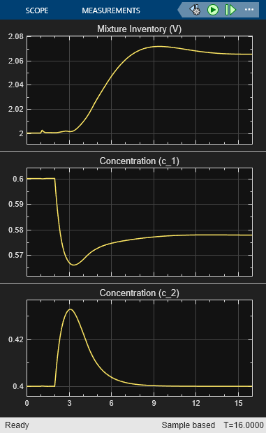
In the simulation:
At time 0, the plant operates steadily at the nominal conditions.
At time 1, the demand decreases by 10%, and the controller maintains the inventory at its setpoint (V=2).
At time 2, there is an unmeasured change in the concentration of both constituents in input feed 1 and of constituent 1 in input feed 3. This disturbance causes a prediction error and a large disturbance in the output blend concentration.
The linear MPC controller recovers well and tries to drive the output blend concentration back to its setpoint. However, after the input feed 1 reaches it upper bound (F_1=1.6), enforced by the custom input/output constraint, the controller can no longer maintain zero steady state error. With the constraint included, the controller does its best given the physical limits of the system.
bdclose(mdl)