R2024b

New Features, Compatibility Considerations

 3-D Truncated Signed Distance Map: Create truncated signed distance maps over voxelized 3-D space

Use the signedDistanceMap3D object to create and store truncated signed distance fields (TSDF) over voxelized 3-D space. You can use the insertPointCloud function to quickly construct your environments in the signed distance map using sensor readings. Using signedDistanceMap3D enables optimization-based motion planners to understand and navigate the environment more effectively, making it easier to avoid obstacles and plan more efficiently.

The first figure shows a reference STL that was used to create point cloud data. The second figure shows a 3-D TSDF generated from the point cloud data. The third figure shows the mesh generated from that 3-D TSDF.
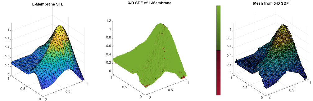
L-membrane STL, a 3-D TSDF generated from L-membrane point cloud data, and a generated mesh from the TSDF

 Factor Graph: Retrieve state covariance from nodes in factor graph

Use the nodeCovariance function to retrieve stored state covariance from a factor graph after optimization. Specify a factorGraphSolverOptions and set the StateCovarianceType property to specify one or more node types for which to estimate and store the state covariance.

The covariance represents the uncertainty associated with the estimated states, which can help you understand the reliability of the state estimates and make informed decisions based on the level of confidence in each estimated state. Incorporating the covariance matrix in state estimation also helps you filter out measurement noise and outliers, thereby improving the overall accuracy and robustness of the estimates.

This figure shows the node state covariances for SE(2) nodes using a helper function. The plotted covariance increases due to drift accumulation with each consecutive node and lowers near loop closures due to the additional state information provided by the loop closure.
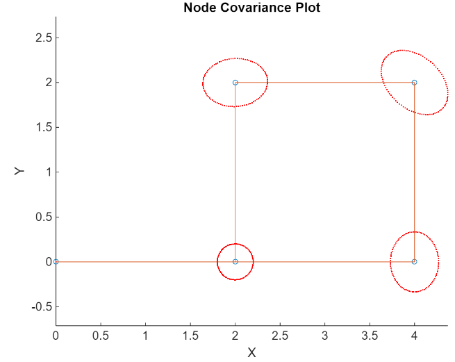
Node state covariance plotted on a simple factor graph.

Path Planning: Shorten paths by removing redundant nodes

Use the shortenpath function to remove redundant nodes along a path between a start point and goal point.

skyplot Function: Specify the status of multiple satellites

The status argument of the skyplot function now accepts structure arrays, enabling you to specify the status of more than one satellite.

 Controller VFH: show now plots on PolarAxes instead of Axes

The show object function of the controllerVFH System object™ now plots on a PolarAxes object instead of an Axes object. The value types of the parent and h arguments reflect this change. See PolarAxes Properties for more information about PolarAxes objects.

timescope Object Enhancements

New color and styling properties for timescope object

You can now customize the plot line, axes, and background color and style settings of the timescope object through the MATLAB® command line.

Higher display precision in timescope UI

You can now increase the display precision to 15 digits using the Display Precision parameter in the Time Scope settings under Display and Labels. This precision affects all the measurement data and the data the scope displays on its status bar.

To open the Time Scope settings, create a timescope object, open its UI, and click Settings in the Scope tab of the toolstrip.

Preserve Colors is now available in Time Scope toolstrip

The Preserve colors for copy to clipboard parameter has been renamed to Preserve Colors, and is now available in the Time Scope toolstrip under Copy Display.

plannerHybridAStar Object: Improved performance

The plan object function of the plannerHybridAStar object shows improved performance. The performance improvement increases as the complexity of the problem increases such as more obstacles. For example, this code is about 3x faster than in the previous release:

function timingTest
    load parkingMap.mat
    map = binaryOccupancyMap(map,3); % Set resolution to 3 cells/metre
    ss = stateSpaceSE2([map.XWorldLimits; map.YWorldLimits; [-pi pi]]);
    sv = validatorOccupancyMap(ss,Map=map);
    planner = plannerHybridAStar(sv,MinTurningRadius=4,MotionPrimitiveLength=6,NumMotionPrimitives=101);
    startPose = [2 9 0];
    goalPose = [27 18 -pi/2];
    path = plan(planner,startPose,goalPose);
end

The approximate execution times are:

  • R2024a: 0.12 s

  • R2024b: 0.04 s

The code was timed on a Windows® 11, AMD Epyc® 74F3 24-Core Processor CPU @ 3.19 GHz test system using the timeit function.

timeit(@timingTest)

controllerTEB Object: Improved performance

The step object function of the controllerTEB object shows improved performance. The performance improvement increases as the complexity of the problem increases such as more obstacles or a higher lookahead time. For example, this code is about 1.5x faster than in the previous release:

function timingTest
    map = load("exampleMaps.mat").complexMap;
    map = binaryOccupancyMap(map); % Default resolution 1 cell/metre
    map = binaryOccupancyMap(map,10); % Increase resolution to 10 cells/metre
    refpath = [6,3,1.57; 8.9,7,0.7; 13.8,10.4,1.07;14.2,11.3,1.57;
              14.2,12.3,2.07;5.08,19.7,1.82; 4.8,20.7,1.3; 9.2,28,0.57;
              29.6,30.8,0.32; 30.5,31.1,0.66; 32,32,-3.1];
    teb = controllerTEB(refpath,map,LookAheadTime=10);
    currentState = refpath(1,:);
    currentVel = [0,0];
    [velcmds,timestamps,optpath] = step(teb,currentState,currentVel);
end

The approximate execution times are:

  • R2024a: 0.37 s

  • R2024b: 0.25 s

The code was timed on a Windows 11, AMD Epyc® 74F3 24-Core Processor CPU @ 3.19 GHz test system using the timeit function.

timeit(@timingTest)

Euler Angle Conversions: Convert to and from other rotations using additional Euler angle sequences

The Coordinate Transformation Conversion block and quat2eul function now support additional Euler sequences. These are all of the supported Euler sequences:

  • "ZYX"

  • "ZYZ"

  • "ZXY"

  • "ZXZ"

  • "YXY"

  • "YZX"

  • "YXZ"

  • "YZY"

  • "XYX"

  • "XYZ"

  • "XZX"

  • "XZY"