Reduce Zero Crossings
Why Reduce Zero Crossings?
Real-time deployment requires using a fixed-step solver. You typically use a variable-step solver for desktop simulation. Variable-step solvers take smaller steps when they detect a zero-crossing event. Smaller steps help to capture the dynamics that cause the zero crossing accurately. Fixed-step solvers do not vary the size of the steps that they take. If your model relies heavily on detecting zero crossings, you might need to specify a very small fixed-step size to capture the dynamics accurately. A small step size can lead to overruns during real-time simulation. By reducing the number of zero crossings, you can configure your solver to use a larger step size for both variable-step and fixed-step deployment while generating results that are accurate enough.
Obtain Reference Results and Plot Simulation Step Size
Simulate your model to generate data that you can use to:
Decide which model elements to change to reduce the number of zero-crossing events.
Assess the accuracy of your modified model.
To open the model, at the MATLAB® command prompt, enter:
model = 'ssc_pneumatic_rts_stiffness_redux';
open_system(model)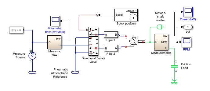
Simulate the model:
sim(model)
Save the data to the workspace.
simlogRef = simlog;
timeRef = tout;
Plot the step size against the simulation time.
h1 = figure;
semilogy(timeRef(1:end-1),diff(timeRef),'-x')
title('Solver Step Size')
xlabel('Time (s)')
ylabel('Step Size (s)')
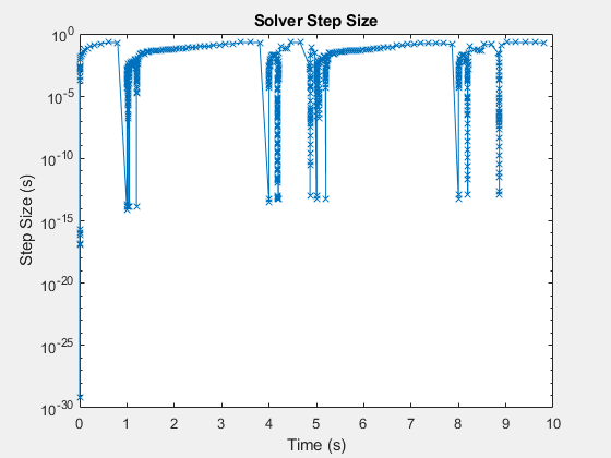
The simulation slows down repeatedly at the beginning of the simulation and at time t = ~1, 4, 5, 8, and 9 seconds.
Zoom to examine the data between time t = 0.8 and 1.03 seconds.
h1;
xStart = 0;
xEnd = 10;
yStart = 0;
yEnd = 10e0;
xZoomStart1 = 0.8;
xZoomEnd1 = 1.03;
yZoomStart1 = 10e-20;
yZoomEnd1 = 10e-1;
axis([xZoomStart1 xZoomEnd1 yZoomStart1 yZoomEnd1])
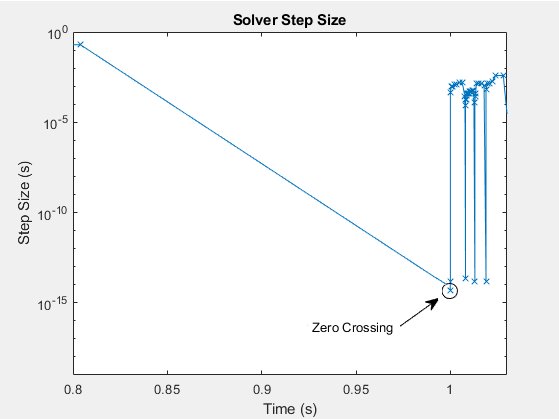
The blue
xmarkers in the figure indicate that the simulation has completed executing a step. The circled markers indicate a very small step size and represent zero-crossing events. The step size decreases to approximately 10e-15 seconds for each zero-crossing detection.To obtain the reference results for motor speed, open the Measurements subsystem. Select the Ideal Rotational Motion Sensor block,
 . With the block selected, use the
simscape.logging.findNodefunction to find and save the node that contains the data forW, the signal for the angular velocity of the motor.nRef = simscape.logging.findNode(simlogRef,gcbh)
nRef =

  Node with properties:

            id: 'Ideal_Rotational_Motion_Sensor'
       savable: 1
    exportable: 0
           phi: [1×1 simscape.logging.Node]
             C: [1×1 simscape.logging.Node]
             R: [1×1 simscape.logging.Node]
             A: [1×1 simscape.logging.Node]
             w: [1×1 simscape.logging.Node]
             t: [1×1 simscape.logging.Node]
             W: [1×1 simscape.logging.Node]
Use the
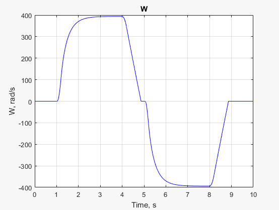
simscape.logging.plotfunction to plot the reference results forW.simscape.logging.plot(nRef.W);
Identify and Modify Elements That Cause Zero Crossings
Analyze the simulation data to determine the elements responsible for the zero crossings. Modify the model to reduce the number of zero crossings that those elements cause.
Use the Simscape™
sscprintzcsfunction to print zero-crossing information for logged simulation data.sscprintzcs(simlogRef)
The results show that the 50 detected zero crossings occur in the Directional 5-way valve block (46 crossings) and the Pneumatic Motor block (4 crossings).ssc_pneumatic_rts_stiffness_redux (42 signals, 50 crossings) +-Directional_5_way_valve (38 signals, 46 crossings) | +-Variable_Area_Orifice_1 (9 signals, 13 crossings) | +-Variable_Area_Orifice_2 (9 signals, 10 crossings) | +-Variable_Area_Orifice_3 (9 signals, 14 crossings) | +-Variable_Area_Orifice_4 (11 signals, 9 crossings) +-Pipe_1 (2 signals, 0 crossings) | +-Constant_Chamber (2 signals, 0 crossings) +-Pneumatic_Motor (2 signals, 4 crossings)
Use the
sscexplorefunction to open the Simscape Results Explorer to interact with logged simulation data.sscexplore(simlogRef)
In the results tree, click Pneumatic Motor to see the results for the motor.
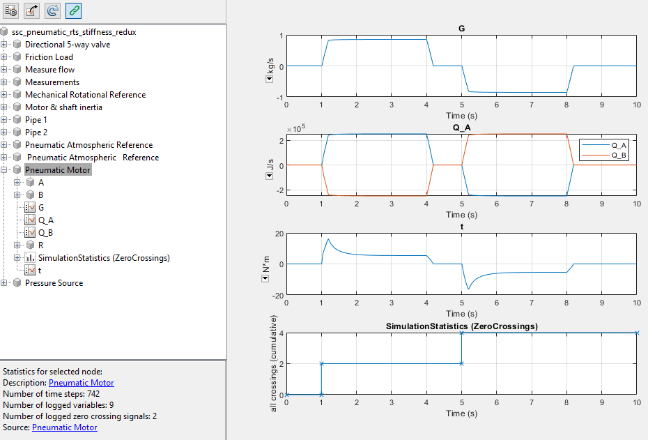
Most of the zero crossings occur between t = 0 and t =1 seconds, when the other signals in the block are near zero. The few remaining zero crossings occur at approximately t = 5 seconds.
To identify the source code that triggers some of the zero crossings, select Directional 5-way valve > Variable Area Orifice 2 > SimulationStatistics (ZeroCrossings) >
 zc_1 - 8 crossings. Click the
Pneumatic.Elements.VariableOrifice link that
appears in the lower, left corner of the window.
zc_1 - 8 crossings. Click the
Pneumatic.Elements.VariableOrifice link that
appears in the lower, left corner of the window.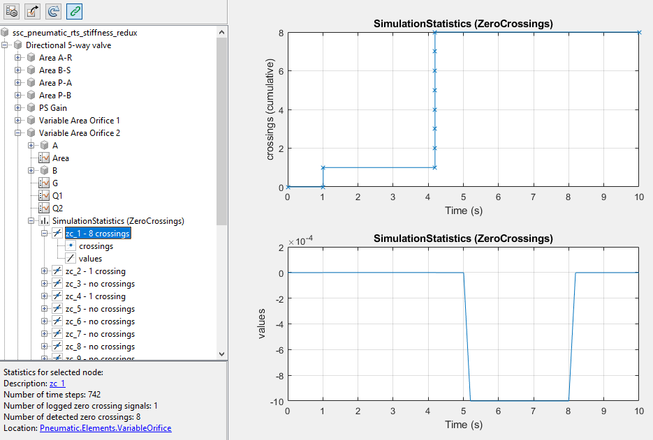
The source code for the Pneumatic Motor block opens with the cursor at this code:
% Area - limit to be greater than Area0
AreaL = if Area<Area0, Area0 else Area end;
The conditional statement that is responsible for the zero crossings is related to the orifice area.
Decrease the number of zero crossings, by decreasing the maximum orifice area of the Directional 5-way valve. Open the Directional 5-way valve block property inspector and specify
995for the Maximum orifice area (mm^2) parameter.
Analyze the Results of the Modified Model
Compare the results to the reference results to ensure the accuracy of your modified model. Confirm that your modified model has fewer zero crossings.
Simulate the model and print the zero crossing data.
sim(model)
sscprintzcs(simlog)
ssc_pneumatic_rts_stiffness_redux (42 signals, 30 crossings)
  +-Directional_5_way_valve (38 signals, 26 crossings)
  | +-Variable_Area_Orifice_1 (9 signals, 7 crossings)
  | +-Variable_Area_Orifice_2 (9 signals, 6 crossings)
  | +-Variable_Area_Orifice_3 (9 signals, 8 crossings)
  | +-Variable_Area_Orifice_4 (11 signals, 5 crossings)
  +-Pipe_1 (2 signals, 0 crossings)
  | +-Constant_Chamber (2 signals, 0 crossings)
  +-Pneumatic_Motor (2 signals, 4 crossings)
The overall number of zero crossings has decreased from 50 to 30.
Compare the results using the
simscape.logging.plotfunction to plot the reference results and the results from the modified model to a single plot:simscape.logging.plot... ({simlogRef.Measurements.Ideal_Rotational_Motion_Sensor.W... simlog.Measurements.Ideal_Rotational_Motion_Sensor.W}, ... 'names', {'Reference','Modified'})
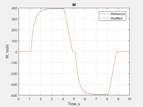
The results look the same.
Zoom control for a closer look at the inflection point at t = ~ 5 seconds.
xStart = 0;
xEnd = 10;
yStart = -400;
yEnd = 400;
xZoomStart1 = 4.75;
xZoomEnd1 = 5.15;
yZoomStart1 = -20;
yZoomEnd1 = 30;
axis([xZoomStart1 xZoomEnd1 yZoomStart1 yZoomEnd1])
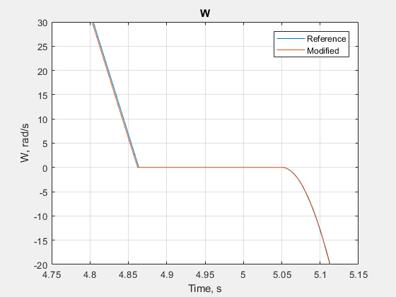
At this zoom level, you can see a small difference in the results for the modified model. However the simulation is accurate enough that the results meet expectations based on empirical and theoretical data.
To improve simulation speed further before performing the real-time simulation workflow with this model, try:
Repeating the method shown in this example to identify and adjust other elements that cause zero crossings that are responsible for the small steps
Reducing any numerical stiffness that is responsible for the small steps
See Also
simscape.logging.plotxy | simscape.logging.findNode | sscexplore | sscprintzcs | Simscape
Results Explorer
Related Examples
- Determine Step Size
- Estimate Computation Costs
- Reduce Computation Costs
- Reduce Fast Dynamics
- Reduce Numerical Stiffness
- Log, Navigate, and Plot Simulation Data
More About
You can also select a web site from the following list:
Americas
- América Latina (Español)
- Canada (English)
- United States (English)
Europe
- Belgium (English)
- Denmark (English)
- Deutschland (Deutsch)
- España (Español)
- Finland (English)
- France (Français)
- Ireland (English)
- Italia (Italiano)
- Luxembourg (English)
- Netherlands (English)
- Norway (English)
- Österreich (Deutsch)
- Portugal (English)
- Sweden (English)
- Switzerland
- United Kingdom (English)