Predict Surface Clutter Power in Range-Doppler Space
This example shows how to calculate the radar cross section (RCS) of a flat featureless surface in range-Doppler space. You will see how to work with the surface RCS to examine the presentation of clutter, analyze the detectability of surface targets, and estimate the total clutter power in a resolution cell by using approximate resolution cell centroids.
Doppler-Processed Clutter Returns
This section introduces the concept of Doppler-processed surface clutter returns and the clutterSurfaceRangeDopplerRCS function, which computes the RCS of clutter in a set of range-Doppler cells. This function expands upon the clutterSurfaceRCS function by computing how clutter returns are distributed over Doppler in addition to range. The function is limited to flat-Earth models with a smooth surface where the normalized RCS (NRCS) can be specified as a function of range.
Range-Doppler Cells
A pulse-Doppler radar system uses a series of coherent pulses to measure the Doppler frequency of a return signal. A set of range gates are used to bin received energy according to range, and a set of Doppler filters are used to bin received energy according to the Doppler frequencies of the signal. This forms a discrete two-dimensional range-Doppler map (RDM) of the received energy. Each pixel of this map corresponds to a range-Doppler cell - a region in space demarcated by two iso-range spheres and two iso-Doppler cones. The intersection of this 3-dimensional region with the surface defines a surface clutter range-Doppler cell whose size corresponds to the amount of received energy in the corresponding pixel of the RDM.
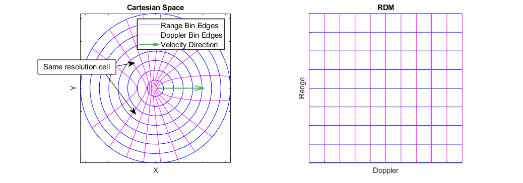
The above figure illustrates the mapping of range-Doppler cells from Cartesian space to the RDM. Note that the distribution of range-Doppler cells is symmetric across the radar's velocity. As a result, most of the range-Doppler cells consist of two disjoint regions in Cartesian space.
Clutter Presentation
This section demonstrates workflows for using the output of clutterSurfaceRangeDopplerRCS to examine how surface clutter is presented in an RDM. You will see how to find the overall range and Doppler extent of the surface, the range and Doppler extent of a conical beam, and how to quickly estimate the Doppler bandwidth of clutter as a function of range.
The Surface in Range-Doppler Space
Surface clutter is distributed over range starting at the range to the nadir point (the radar altitude) out to the horizon. It is also distributed over 360 degrees of azimuth angle and up to 90 degrees of elevation angle. The large angular spread of surface clutter causes it to be distributed over a range of Doppler frequencies as well. Understanding where surface clutter will appear in a set of range-Doppler cells, and how much of the surface contributes to each cell, is important for many applications including control system design and detectability analysis. Typical radar antennas use a tight beam to isolate small regions of the surface, and in this example you will see how to incorporate radar beam information into the analysis of clutter return. In this analysis, a flat-Earth assumption is used and as such, surface clutter is unbounded in range. The interval of ranges covered is then , but a maximum range of interest can be specified.
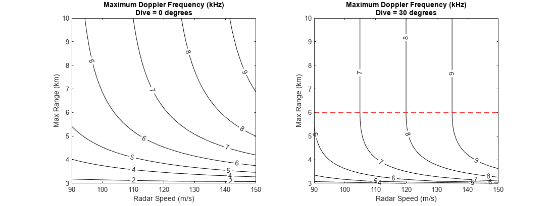
Unlike range, the Doppler frequency of surface clutter will always be bounded and may be limited either by the maximum range sampled by the radar or by the speed of the radar. Besides the total speed of the radar, the z-component of the radar's velocity must be known, which is captured by the dive angle - the angle of the velocity vector with the horizontal, with positive dive indicating the velocity is pointing down.
The function helperSurfaceDopplerLimits is provided to calculate the min and max Doppler of surface clutter, and the figure below shows the maximum surface Doppler as a function of radar speed and max range for a 10 GHz radar at an altitude of 3 km. When the dive angle is nonzero, there will be a critical range (indicated as a red dashed line in the right subplot) at which the velocity vector intersects the surface, above which the maximum Doppler depends only on the radar speed.
freq = 10e9; % Hz
alt = 3e3;   % m
helperSurfaceDopplerLimitsChart(freq,alt)
Run the clutterSurfaceRangeDopplerRCS function to see the surface RCS. Start by defining the required system and platform parameters. Use a 78 Hz Doppler resolution, and let the platform travel at 120 m/s with a dive angle of 10 degrees.
dopres = 78; % Hz
speed = 120; % m/s
dive = 10;   % deg
Define a range swath that starts at 5 km, covering 5 km of range at a 40 m resolution. This defines the centers of each slant range bin.
R = 5e3:40:10e3;
Create a surfaceReflectivityLand object for getting the required NRCS values. The Barton model for flat land surfaces is used by default. Use the grazingang function to find the grazing angles corresponding to each range, then get the NRCS at each range.
graze = grazingang(alt,R,"Flat");
refl = surfaceReflectivityLand;
nrcs = refl(graze,freq);
Compute the RCS of clutter over the specified range swath and use the provided helper function to plot the results.
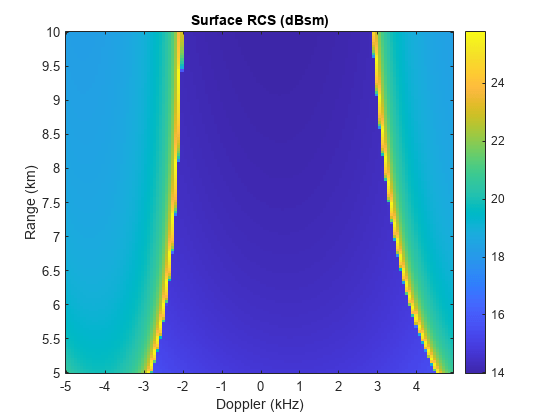
[rcs,dop] = clutterSurfaceRangeDopplerRCS(nrcs,R,freq,dopres,alt,speed,dive);
helperPlotSurfaceRCS(R,dop,rcs)
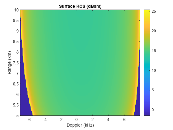
Some interesting things can be observed in this result:
The nonzero dive angle results in the clutter return being skewed slightly towards higher Doppler at lower ranges and lower Doppler at higher ranges.
The Doppler extent of surface clutter increases with range
The clutter around 0 Hz, corresponding to the broadside direction, shows an RCS that changes only slightly with range
The clutter return at the min and max Doppler in each range gate is spikier and less predictable
The Beam Footprint in Range-Doppler Space
The previous section looked at the overall extent of the surface in range-Doppler space, but to understand the whole story, the radar beam should be considered as well.
The clutterSurfaceRangeDopplerRCS function will compute the RCS of clutter over all 360 degrees of azimuth and does not consider limiting by a radar beam. For a simple conical beam defined by an azimuth and elevation beamwidth, the min and max range of the beam footprint and the min and max Doppler cone inside the beam can be calculated in closed form. This information may be used in tandem with the output from clutterSurfaceRangeDopplerRCS to determine the RCS of clutter that falls within the beam.
The function helperConicalBeamLimits is provided to compute the extent of the beam footprint in range-Doppler space for a simple symmetric conical beam. The figure below shows how the min and max Doppler limits of the beam footprint change with azimuth angle relative to broadside (sometimes referred to as ground-plane squint angle) for two different dive angles. Use a beam with a 10 degree beamwidth pointed down at 30 degrees.
beamw = 10; % deg
dep = 30;   % deg
helperBeamDopplerLimitsChart(freq,alt,speed,beamw,dep)
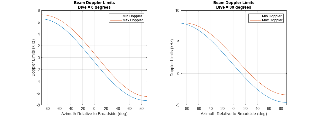
The above figure illustrates that, with a level flight path, the beam always covers the same range of Doppler frequencies, and the broadside direction centers the beam on 0 Hz. With a 30 degree dive angle, the extent of the beam in Doppler varies depending on azimuth pointing.
The range and Doppler limits of the beam footprint can be used to extract the surface RCS that falls within the beam. Let the radar beam point in the broadside direction at the 30 degree depression angle specified earlier.
az = 0; % deg
[R1,R2,d1,d2] = helperConicalBeamLimits(freq,alt,speed,dive,beamw,az,dep)
R1 = 5.2303e+03
R2 = 7.0986e+03
d1 = -2.6652
d2 = 1.3875e+03
R1 and R2 are the min and max slant ranges to the beam footprint (in meters), and d1 and d2 are the min and max Doppler frequencies of the footprint (in Hz).
Plot the surface RCS again, showing the region within these range and Doppler limits.
helperPlotSurfaceRCS(R,dop,rcs,R1,R2,d1,d2)
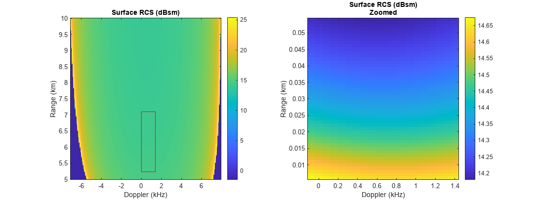
In this nice broadside case, the surface RCS within the beam shows only a slight variation with Doppler and varies only by about 0.4 dBsm across the beam.
Now try an off-broadside beam geometry. Set the azimuth relative to broadside to -60 degrees (pointing towards the direction of motion) and plot the results again.
az = -60; % deg
[R1,R2,d1,d2] = helperConicalBeamLimits(freq,alt,speed,dive,beamw,az,dep);
helperPlotSurfaceRCS(R,dop,rcs,R1,R2,d1,d2)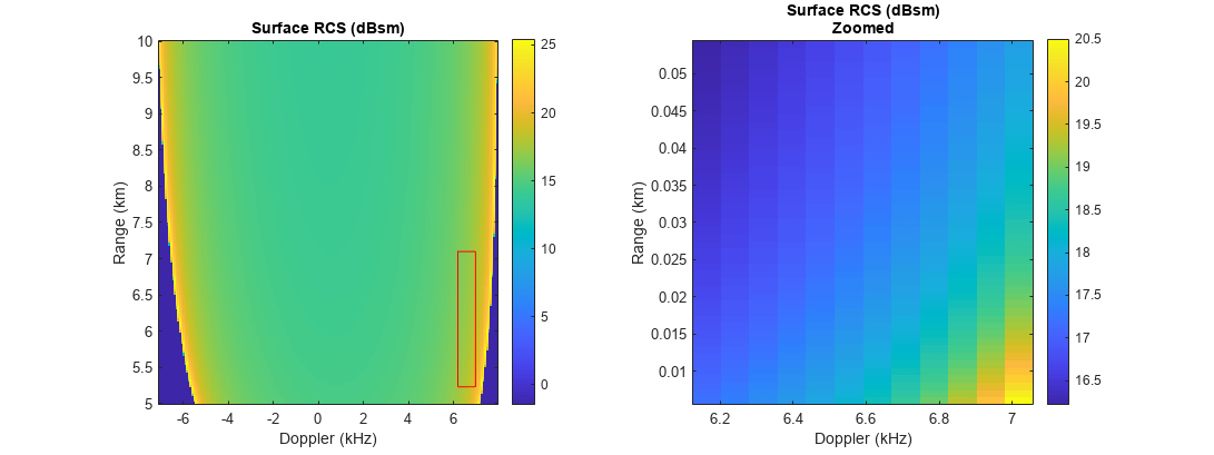
In this squinted case, the surface RCS varies significantly with both range and Doppler, and shows about a 4 dBsm variation across the beam. Such variation can cause trouble for detection algorithms and gain control.
Doppler Bandwidth
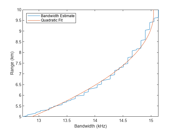
The total Doppler bandwidth of clutter at a given range is an important metric in applications such as receiver chain design, PRF selection, and MTI filter design. The range-Doppler map of surface RCS can be used to find the Doppler extent of clutter in each range bin.
Loop over range bins and, for each range, find the first and last Doppler bins with nonzero RCS. Estimate the bandwidth as the number of bins covered times the Doppler resolution. This approximation is a baseline that can be expanded upon to incorporate information about things like Doppler sidelobes and intrinsic clutter motion.
bandw = zeros(1,numel(R));
for gIdx = 1:numel(R)
    I1 = find(rcs(gIdx,:),1,'first');
    I2 = find(rcs(gIdx,:),1,'last');
    bandw(gIdx) = (I2 - I1 + 1)*dopres;
end
Find a quadratic fit and plot the results.
pf = polyfit(R,bandw,2);
figure
plot(bandw/1e3,R/1e3)
hold on
plot(polyval(pf,R)/1e3,R/1e3);
hold off
xlabel('Bandwidth (kHz)')
ylabel('Range (km)')
legend('Bandwidth Estimate','Quadratic Fit','Location','northwest')
set(gca,'XLimitMethod','tight')
Doppler Wrapping
Coherent radar pulses are collected at a constant rate, known as the pulse-repetition frequency (PRF), over the course of a coherent processing interval (CPI). The pulses are stored in a matrix sometimes referred to as a data cube or phase history (PH), which gives a range-time map of received energy. Doppler processing is implemented in modern digital systems with a slow-time (across pulses) fast Fourier transform (FFT). As such, the Doppler spectrum of the return signal is subject to wrapping around a frequency interval of length PRF. This means that the apparent distribution of clutter returns in Doppler may be quite complex, and it's possible for a pixel of the RDM to contain return from multiple range-Doppler cells at congruent Doppler frequencies.
helperDopplerWrappingExample
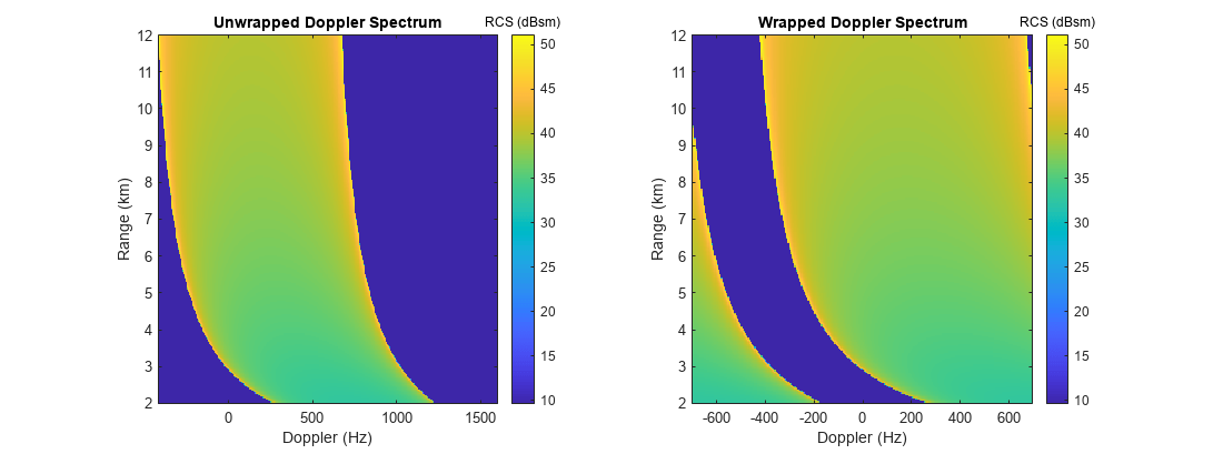
It can be useful to examine the unwrapped Doppler spectrum of clutter. For example, to see how various fast-time filters in the receiver chain might affect the clutter return signal. It is also useful to examine the wrapped Doppler spectrum to see how much total clutter return appears in a given pixel of the RDM. The clutterSurfaceRangeDopplerRCS function can do both. Doppler wrapping is enabled by specifying the number of Doppler bins to use via the optional NumDopplerBins parameter. No wrapping due to ambiguous ranges is performed.
Start by specifying the number of Doppler bins to use.
numdop = 128;
Find the PRF that is implied by this specification using the Doppler resolution that was specified earlier.
prf = dopres*numdop
prf = 9984
Call the function as before, but this time specify the number of Doppler bins to use. The resulting clutter RCS will be centered about 0 Hz and extend over the interval .
[rcs,dop] = clutterSurfaceRangeDopplerRCS(nrcs,R,freq,dopres,alt,speed,dive,'NumDopplerBins',numdop);Plot the result.
helperPlotSurfaceRCS(R,dop,rcs)
Since the PRF is lower than the minimum Doppler bandwidth over the range swath and because no limiting by the beam is considered here, the clutter return will fill the entire RDM. Ridges corresponding to the min and max unwrapped Doppler are still visible.
Analyze the Detectability of Surface Targets
In this section, you will see how to use clutterSurfaceRangeDopperRCS to make a rough determination of the detectability of a surface target based on its RCS. Assume that the beam is pointing at the target and that the gain does not vary significantly over a resolution cell. With this assumption, the signal-to-clutter ratio (SCR) can be found from the ratio of target RCS to clutter RCS in the resolution cell that contains the target.
Start by defining collection parameters for a typical airborne pulse-Doppler radar system. Use a 10 GHz frequency, a range resolution of 80 m, and a 31 Hz Doppler resolution. The range swath will start at 10 km and cover 400 range gates.
freq = 10e9;       % Hz
rngres = 80;       % m
dopres = 31;       % Hz
startrange = 10e3; % m
numrange = 400;
R = startrange + (0:numrange-1)*rngres;
Position the radar at an altitude of 4 km above the origin, flying horizontally in the +X direction at 240 m/s.
alt = 4e3;   % m
speed = 240; % m/s
dive = 0;    % deg
Now define the target. Place it on the surface at a range of 14 km in the broadside direction. Let the target have an RCS of 6 dBsm.
tgtrng = 14e3; % m
tgtgndrng = sqrt(tgtrng^2-alt^2);
tgtpos = [0 tgtgndrng 0];
tgtrcs = 6; % dBsm
Calculate the Doppler frequency of the target.
rdrpos = [0 0 alt];
rdrvel = speed*[cosd(dive) 0 -sind(dive)];
lambda = freq2wavelen(freq);
tgtdop = 2/lambda*dot(rdrvel,tgtpos-rdrpos)/tgtrng
tgtdop = 0
Since the target lies in the broadside direction and the radar is not diving, the Doppler frequency of the target is 0 Hz.
Compute the surface RCS. Use the same reflectivity model as earlier.
graze = grazingang(alt,R,"Flat");
nrcs = refl(graze,freq);
[rcs,dop] = clutterSurfaceRangeDopplerRCS(nrcs,R,freq,dopres,alt,speed,dive);
Recall that the surface RCS in each range-Doppler cell returned by clutterSurfaceRangeDopplerRCS includes clutter return from the full 360 degrees of azimuth. As such, with the assumption that the surface returns are limited by a beam that only intersects the resolution cell on one side of the radar velocity vector, the surface RCS within the beam is half of the value returned by clutterSurfaceRangeDopplerRCS. Divide the RCS by two now.
rcs = rcs/2;
Extract the surface RCS in the 0 Hz Doppler bin.
rcs0Hz = rcs(:,dop==0);
Find the range bin containing the target and the surface RCS at the target range. Estimate the SCR (in dB) by finding the difference between the target and surface RCS.
[~,tgtrngbin] = min(abs(tgtrng-R));
surfrcs = pow2db(rcs0Hz(tgtrngbin));
tgtscr = tgtrcs - surfrcs
tgtscr = -2.1058
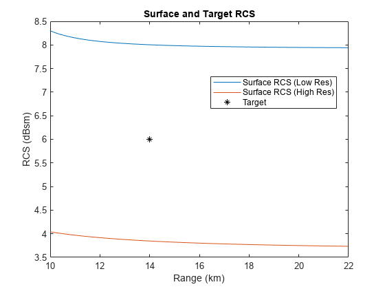
With a negative SCR, the target is unlikely to be detected. Now try decreasing the range resolution to 30 m and repeat the experiment.
rngres = 30; % m
R = startrange + (0:numrange-1)*rngres;
graze = grazingang(alt,R,"Flat");
nrcs = refl(graze,freq);
[rcs,dop] = clutterSurfaceRangeDopplerRCS(nrcs,R,freq,dopres,alt,speed,dive);
rcs = rcs/2;
rcs0Hz_highRes = rcs(:,dop==0);
[~,tgtrngbin] = min(abs(tgtrng-R));
surfrcs = pow2db(rcs0Hz_highRes(tgtrngbin));
tgtscr = tgtrcs - surfrcs
tgtscr = 2.1536
With the improved range resolution, the size of the range-Doppler cell on the ground is smaller, resulting in less reflected power from the surface, and the target may be detected. This assumes the entire target falls within one range resolution cell and that range straddling is not significant. Use the provided helper function to plot a visualization of the surface RCS at both range resolutions along with the target.
helperPlotSurfTgtRCS(R,rcs0Hz,rcs0Hz_highRes,tgtrng,tgtrcs)
Estimate Clutter Power and Returns
In this section you will see how to quickly generate clutter returns using the clutter RCS information along with an estimate of the centroids of the range-Doppler cells on the surface. You will treat each centroid as a point target with an RCS equal to that of the corresponding cell, use the radar equation to find the received clutter power in each cell, then construct the slow-time signal with phase noise and thermal noise.
Compute Clutter Power
Start by defining the radar system parameters. Use a 2.4 GHz frequency, 80 m range resolution, a PRF of 6 kHz, and 128 Doppler bins (which will correspond to 128 pulses). The NumDopplerBins parameter will be used again to get a DC-centered Doppler spectrum.
freq = 2.4e9; % Hz
rngres = 80;  % m
prf = 6e3;    % Hz
numdop = 128;
Find the Doppler resolution of this system.
dopres = prf/numdop;
Place the radar at an altitude of 4 km, traveling at 100 m/s with a slight 10 degree dive.
alt = 4e3;   % m
speed = 100; % m/s
dive = 10;   % deg
Define a range swath that starts at the nadir point and covers 120 gates.
startrange = alt;
numrange = 120;
R = startrange + (0:numrange-1)*rngres;
This particular workflow requires that the clutter bandwidth not exceed the PRF, which can be checked with the provided helper function.
[d1,d2] = helperSurfaceDopplerLimits(freq,alt,speed,dive,R(end));
d2 - d1 < prf
ans = logical
   1
If the Doppler bandwidth does exceed the PRF, Doppler wrapping could be performed after calculating the clutter power in each cell of the unwrapped spectrum.
Calculate the NRCS of the surface in each range bin using the reflectivity model created earlier.
graze = grazingang(alt,R,"Flat");
nrcs = refl(graze,freq);
In order to generate a more realistic clutter signal, enable Weibull speckle on the reflectivity model using a shape parameter of 0.8, and generate a new instance of speckle for each Doppler bin.
release(refl)
refl.Speckle = "Weibull";
refl.SpeckleShape = 0.8;
spck = zeros(numrange,numdop);
for ind = 1:numdop
    [~,spck(:,ind)] = refl(graze,freq);
end
Compute the surface RCS for the given parameters. Multiply-in the speckle values, and once again divide the returned RCS by two to get the RCS on one side of the radar velocity vector.
[rcs,dop] = clutterSurfaceRangeDopplerRCS(nrcs,R,freq,dopres,alt,speed,dive,'NumDopplerBins',numdop);
rcs = rcs.*spck;
rcs = rcs/2;
Define the radar look direction. Point the radar in the broadside direction (90 degrees, relative to the velocity vector) and down by 30 degrees.
azLook = 90;  % deg, relative to velocity vector
elLook = -30; % deg
The helperRangeDopplerCellCenters function is provided to find the coordinates of the range-Doppler cell centers on the surface, which approximates the power centroid for each cell. This function assumes the radar is positioned above the origin and is traveling in the +X direction. The returned coordinate values will be NaN for cells whose centers do not intersect the surface.
lambda = freq2wavelen(freq);
[cx,cy] = helperRangeDopplerCellCenters(R,dop,lambda,alt,speed,dive);
Plot the computed centroid positions using the provided helper function.
helperPlotCellCentroids(cx,cy)
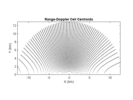
Only the cells in the +Y half of the plane are considered, since that is the direction the radar is pointed.
Find the lines of sight (LOS) from the radar to the centroids, convert them to the sensor frame, and get the angles to each cell in the sensor frame.
sensorFrame = rotz(azLook)*roty(-elLook);

% Lines of sight to centroids in scenario frame
losx = cx;
losy = cy;
losz = -alt;

% Convert to sensor frame
[losx,losy,losz] = deal(sensorFrame(1,1)*losx+sensorFrame(2,1)*losy+sensorFrame(3,1)*losz,...
                        sensorFrame(1,2)*losx+sensorFrame(2,2)*losy+sensorFrame(3,2)*losz,...
                        sensorFrame(1,3)*losx+sensorFrame(2,3)*losy+sensorFrame(3,3)*losz);

% Get az/el angles to centroids
[az,el,~] = cart2sph(losx,losy,losz);
az = rad2deg(az);
el = rad2deg(el);
Create a 14-by-14 uniform rectangular array (URA) for computing the antenna gain in the direction of each range-Doppler cell.
array = phased.URA([14 14],lambda/2);
Create a phased.ArrayResponse System object for getting the magnitude response of the array in the direction of each cell centroid. Only input the valid (non-NaN) centroids to the array response and express the results in dB.
antresp = phased.ArrayResponse('SensorArray',array);
nonnan = ~isnan(az) & ~isnan(el);
antGain = zeros(numrange,numdop);
antGain(nonnan) = antresp(freq,[az(nonnan) el(nonnan)].');
antGain = mag2db(abs(antGain));
The radar equation returns signal-to-noise (SNR) ratios, so calculate the noise power now in order to back out the received clutter power. Calculate the pulse width assuming a simple rectangular pulse. Use 290 K for the noise temperature, then find the noise power in dBW.
tau = range2time(rngres);
Ts = 290;
noisePwr = 10*log10(physconst('Boltzmann')*Ts/tau);
Use a 10 kW transmit power.
txPwr = 10e3;
Loop over the range-Doppler cells, and use radareqsnr and the noise power computed earlier to get the expected clutter power in each cell.
clutPwr = -inf(numrange,numdop);
for rIdx = 1:numrange
    for dIdx = 1:numdop
        if rcs(rIdx,dIdx) > 0
            clutPwr(rIdx,dIdx) = radareqsnr(lambda,R(rIdx),txPwr,tau,'RCS',rcs(rIdx,dIdx),'Gain',antGain(rIdx,dIdx),'Ts',Ts) + noisePwr;
        end
    end
end
Plot the results.
imagesc(dop/1e3,R/1e3,clutPwr)
set(gca,'ydir','normal')
xlabel('Doppler (kHz)')
ylabel('Range (km)')
title('Power of Surface Reflection (dBW)')
colorbar
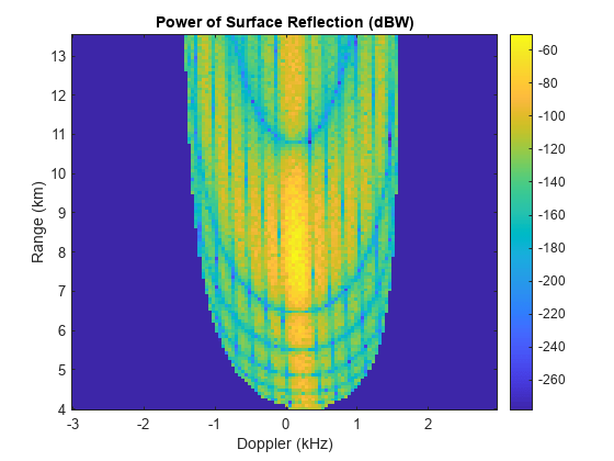
The antenna lobe structure and the effect of the added speckle can be seen clearly in the map of clutter power. Note that this result shows how the power received by reflections off the surface is distributed in range and Doppler but does not include signal processing gains. Speckle could be omitted to get an average clutter power instead.
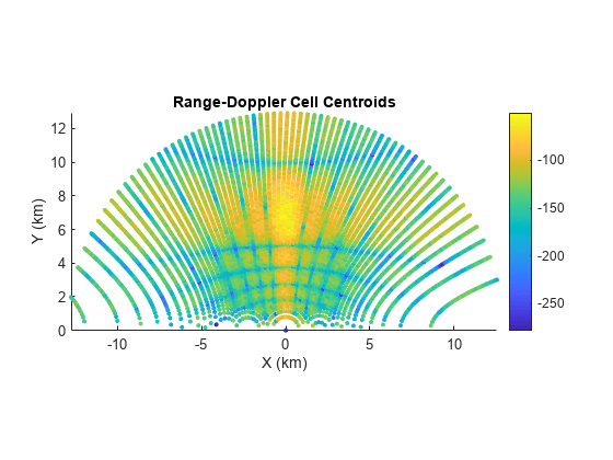
Plot the cell centroids again, but this time color code them to see how the returned power is distributed in Cartesian space.
helperPlotCellCentroids(cx,cy,clutPwr)
Simulate Clutter Returns
A simple clutter return signal can be generated by constructing a slow-time signal with the appropriate power and phase, and adding Doppler sidelobes and thermal noise. Start by converting the clutter power to magnitude values.
clutMag = db2mag(clutPwr);
Use the provided helper function to generate a slow-time signal from the computed magnitude spectrum. This function adds Doppler sidelobes by applying frequency and phase offsets to the signal at each Doppler frequency.
PH = helperFormSlowTimeSignal(clutMag,prf,R);
Add thermal noise. Adjust the noise power to account for the number of independent channels of the array that are summed together.
numchan = getNumElements(array);
noisePwrSum = noisePwr + 10*log10(numchan);
ni = randn(size(PH));
nq = randn(size(PH));
PH = PH + db2mag(noisePwrSum)*(ni+1i*nq)/sqrt(2);
Form the DC-centered RDM
RDM = fftshift(fft(PH,[],2),2);
Plot the resulting RDM. The color scale extends from 20 dBW below the expected noise power in the RDM up to -10 dBW.
imagesc(dop/1e3,R/1e3,20*log10(abs(RDM)))
set(gca,'ydir','normal')
xlabel('Doppler (kHz)')
ylabel('Range (km)')
title('Predicted RDM (dBW)')
colorbar
clim([noisePwrSum-20+20*log10(numdop) -10])
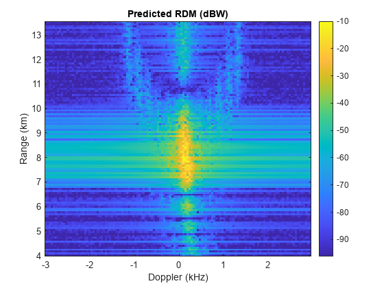
In addition to the Doppler sidelobes, fast-time effects could be accounted for by applying waveform information to each pulse and simulating range sidelobes.
Compare to Radar Scenario
The provided helper function helperCompareToScenario demonstrates how to collect clutter returns for the same scenario parameters using radarScenario. The radar scenario allows flexible clutter simulation with support for any of the available waveform types, realistic platform trajectories, and heterogeneous surfaces (terrain, reflectivity maps, curved-Earth, etc.).
The figure below shows the output that can be expected from the scenario simulation.
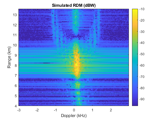
There is a close agreement between these two very different methods of clutter generation.
You can run the scenario simulation as part of this example by uncommenting the line below. The simulation takes 10 to 15 minutes on a machine with 64 GB of RAM and a 3 GHz processor.
%helperCompareToScenario(array,numdop,prf,refl,rngres,freq,azLook,elLook,txPwr,noisePwr,alt,speed,dive,R,dop)Conclusion
In this example you saw how to compute the RCS of a flat surface in range-Doppler space. You saw how to investigate the presentation of surface clutter when interrogated by a conical beam, and how to use the surface RCS in tandem with simple geometric calculations to perform a quick analysis of the detectability of surface targets based on their RCS. Finally, you saw how to quickly estimate clutter power and simulate clutter returns using approximate cell centroids and the radar equation.
Supporting Functions
helperSurfaceDopplerLimitsChart
function helperSurfaceDopplerLimitsChart(freq,alt)
% Create a chart to visualize the Doppler limits of a flat surface.

spd = linspace(90,150,80);
maxRange = linspace(3e3,10e3,80);

dive = 0;
d1_0 = zeros(numel(maxRange),numel(spd));
d2_0 = d1_0;
for spdIdx = 1:numel(spd)
    for rIdx = 1:numel(maxRange)
        [d1_0(rIdx,spdIdx),d2_0(rIdx,spdIdx)] = helperSurfaceDopplerLimits(freq,alt,spd(spdIdx),dive,maxRange(rIdx));
    end
end

dive = 30;
d1_30 = zeros(numel(maxRange),numel(spd));
d2_30 = d1_30;
for spdIdx = 1:numel(spd)
    for rIdx = 1:numel(maxRange)
        [d1_30(rIdx,spdIdx),d2_30(rIdx,spdIdx)] = helperSurfaceDopplerLimits(freq,alt,spd(spdIdx),dive,maxRange(rIdx));
    end
end

critR = alt/sind(dive);

h = figure;
subplot(1,2,1)
contour(spd,maxRange/1e3,d2_0/1e3,[2 4 5 6 7 8 9],'black','showtext','on')
title({'Maximum Doppler Frequency (kHz)';'Dive = 0 degrees'})
xlabel('Radar Speed (m/s)')
ylabel('Max Range (km)')
subplot(1,2,2)
contour(spd,maxRange/1e3,d2_30/1e3,[2 4 5 6 7 8 9],'black','showtext','on')
title({'Maximum Doppler Frequency (kHz)';'Dive = 30 degrees'})
xlabel('Radar Speed (m/s)')
ylabel('Max Range (km)')
line(xlim,[critR critR]/1e3,'color','red','linestyle','--')
h.Position = h.Position + [0 0 560 0];
set(gca,'XLimitMethod','tight')

end
helperPlotSurfaceRCS
function helperPlotSurfaceRCS(R,dop,rcs,R1,R2,d1,d2)
% Plot the RCS of a surface in range-Doppler space. Optionally, zoom in on
% a specified interval.

h = figure;

if nargin > 3
    subplot(1,2,1)
end

imagesc(dop/1e3,R/1e3,10*log10(rcs))
set(gca,'ydir','normal')
xlabel('Doppler (kHz)')
ylabel('Range (km)')
title('Surface RCS (dBsm)')
colorbar

if nargin > 3
    patch([d1 d2 d2 d1]/1e3,[R1 R1 R2 R2]/1e3,'','FaceColor','none','EdgeColor','red')

    subplot(1,2,2)
    RIdx1 = find(R <= R1,1,'last');
    RIdx2 = find(R >= R2,1,'first');
    DIdx1 = find(dop <= d1,1,'last');
    DIdx2 = find(dop >= d2,1,'first');
    imagesc(dop(DIdx1:DIdx2)/1e3,(RIdx1:RIdx2)/1e3,10*log10(rcs(RIdx1:RIdx2,DIdx1:DIdx2)))
    set(gca,'ydir','normal')
    xlabel('Doppler (kHz)')
    ylabel('Range (km)')
    title({'Surface RCS (dBsm)';'Zoomed'})
    colorbar

    h.Position = h.Position + [0 0 560 0];
end

end
helperBeamDopplerLimitsChart
function helperBeamDopplerLimitsChart(freq,alt,spd,bw,dep)
% Create a chart to visualize the Doppler limits of a beam.

az = linspace(-90,90,1e3);

dive = 0;
d1_0 = zeros(1,numel(az));
d2_0 = d1_0;
for ind = 1:numel(az)
    [~,~,d1_0(ind),d2_0(ind)] = helperConicalBeamLimits(freq,alt,spd,dive,bw,az(ind),dep);
end

dive = 30;
d1_30 = zeros(1,numel(az));
d2_30 = d1_30;
for ind = 1:numel(az)
    [~,~,d1_30(ind),d2_30(ind)] = helperConicalBeamLimits(freq,alt,spd,dive,bw,az(ind),dep);
end

h = figure;
subplot(1,2,1)
plot(az,d1_0/1e3,az,d2_0/1e3)
title({'Beam Doppler Limits';'Dive = 0 degrees'})
xlabel('Azimuth Relative to Broadside (deg)')
ylabel('Doppler Limits (kHz)')
legend('Min Doppler','Max Doppler')
grid on
set(gca,'XLimitMethod','tight')
subplot(1,2,2)
plot(az,d1_30/1e3,az,d2_30/1e3)
title({'Beam Doppler Limits';'Dive = 30 degrees'})
xlabel('Azimuth Relative to Broadside (deg)')
ylabel('Doppler Limits (kHz)')
grid on
legend('Min Doppler','Max Doppler')
set(gca,'XLimitMethod','tight')
h.Position = h.Position + [0 0 560 0];

end
helperConicalBeamLimits
function [R1,R2,d1,d2] = helperConicalBeamLimits(freq,alt,spd,dive,bw,az,graze)
% Return the range and Doppler limits of a conical beam footprint.

if graze <= -bw/2
    R1 = inf;
    R2 = inf;
elseif graze <= bw/2
    R1 = alt/sind(graze+bw/2);
    R2 = inf;
elseif graze <= 90-bw/2
    R1 = alt/sind(graze+bw/2);
    R2 = alt/sind(graze-bw/2);
else
    R1 = alt;
    R2 = alt/sind(graze-bw/2);
end

lambda = freq2wavelen(freq);

azVel = az + 90; % use azimuth relative to velocity vector
squint = acosd(cosd(dive)*cosd(azVel)*cosd(graze) + sind(dive)*sind(graze));

if squint <= bw/2
    t1 = squint + bw/2;
    t2 = 0;
else
    t1 = squint + bw/2;
    t2 = squint - bw/2;
end

d1 = 2/lambda*spd*cosd(t1);
d2 = 2/lambda*spd*cosd(t2);

end
helperDopplerWrappingExample
function helperDopplerWrappingExample
% Plot a demonstration of Doppler wrapping

alt = 1e3;
freq = 2e9;
prf = 1.4e3;
ndop = 256;
dopres = prf/ndop;
dive = 70;
speed = 120;

R = 2e3:40:12e3;
nrcs = ones(size(R));

[RCS1,dopbins1] = clutterSurfaceRangeDopplerRCS(nrcs,R,freq,dopres,alt,speed,dive);
[RCS2,dopbins2] = clutterSurfaceRangeDopplerRCS(nrcs,R,freq,dopres,alt,speed,dive,'NumDopplerBins',ndop);

h = figure;
subplot(1,2,1)
imagesc(dopbins1,R/1e3,10*log10(RCS1))
set(gca,'ydir','normal')
title('Unwrapped Doppler Spectrum')
xlabel('Doppler (Hz)')
ylabel('Range (km)')
ch=colorbar;
ch.Title.String='RCS (dBsm)';
subplot(1,2,2)
imagesc(dopbins2,R/1e3,10*log10(RCS2))
set(gca,'ydir','normal')
title('Wrapped Doppler Spectrum')
xlabel('Doppler (Hz)')
ylabel('Range (km)')
ch=colorbar;
ch.Title.String='RCS (dBsm)';
h.Position = h.Position + [0 0 560 0];

end
helperPlotSurfTgtRCS
function helperPlotSurfTgtRCS(R,rcsLow,rcsHigh,tgtrng,tgtrcs)
% Plot RCS against range and annotate the target range and rcs.

plot(R/1e3,10*log10(rcsLow))
hold on
plot(R/1e3,10*log10(rcsHigh))
plot(tgtrng/1e3,tgtrcs,'*black')
hold off
xlabel('Range (km)')
ylabel('RCS (dBsm)')
legend('Surface RCS (Low Res)','Surface RCS (High Res)','Target','Location','best')
title('Surface and Target RCS')

end
helperSurfaceDopplerLimits
function [d1,d2] = helperSurfaceDopplerLimits(freq,alt,spd,dive,maxRange)
% Return the Doppler limits of a flat surface.

% Depression angle to max range
if maxRange < alt
    maxRangeDep = 90;
else
    maxRangeDep = 90 - acosd(alt/maxRange);
end

% Normalized maximum closing rate
if dive < maxRangeDep
    maxClosing = cosd(maxRangeDep-dive);
else
    maxClosing = 1;
end

% Normalized minimum closing rate
if -dive < maxRangeDep
    minClosing = -cosd(maxRangeDep+dive);
else
    minClosing = -1;
end

% Factor in speed and convert to Doppler
lambda = freq2wavelen(freq);
d1 = 2/lambda*spd*minClosing;
d2 = 2/lambda*spd*maxClosing;

end
helperRangeDopplerCellCenters
function [x,y] = helperRangeDopplerCellCenters(R,dop,lambda,alt,speed,dive)
% Return the x/y coordinates of the centers of a set of range-Doppler cells
% on the surface

R = R(:);
dop = dop(:).';

r = sqrt(R.^2-alt^2);
ctheta = (lambda*R.*dop/(2*speed) - alt*sind(dive))./(r*cosd(dive));
ctheta(r == 0,:) = 0;
ctheta(ctheta>1) = nan;
ctheta(ctheta<-1) = nan;
theta = acosd(ctheta);

x = r.*cosd(theta);
y = r.*sind(theta);

end
helperPlotCellCentroids
function helperPlotCellCentroids(cx,cy,cdata)
% Plot cell centroids in Cartesian space. Optionally specify color data.

if nargin < 3
    plot(cx(:)/1e3,cy(:)/1e3,'.black','MarkerSize',1)
else
    scatter(cx(:)/1e3,cy(:)/1e3,10,cdata(:),'filled')
    colorbar
end
title('Range-Doppler Cell Centroids')
xlabel('X (km)')
ylabel('Y (km)')
axis equal
set(gca,'XLimitMethod','tight')
set(gca,'YLimitMethod','tight')

end
helperFormSlowTimeSignal
function PH = helperFormSlowTimeSignal(specmag,prf,R)
% Form a time-domain signal from the magnitude spectrum

[numr,numd] = size(specmag);

% Unshift magnitude spectrum
specmag = ifftshift(specmag,2);

% Initialize time domain signal
PH = zeros(size(specmag));

% Sample times
tslow = 0:1/prf:(numd-1)/prf;
tfast = 2*(R(:)-R(1))/299792458;
t = tslow + tfast;

% Randomized phase offsets for each bin
phi = rand(numr,numd)-1/2;

% Doppler axis
df = prf/numd;
dop = 0:df:(prf-df);

% Random Doppler offsets in each bin
fc = dop + (rand(numr,numd)-1/2)*df;

for ind = 1:numd
    % Entire signal at the current Doppler frequency
    y = specmag(:,ind).*exp(1i*2*pi*(fc(:,ind).*t+phi(:,ind)));

    % Accumulate
    PH = PH + y;
end

end
helperCompareToScenario
function helperCompareToScenario(array,numdop,prf,refl,rngres,fc,azLook,elLook,txPwr,noisePwrDb,alt,speed,dive,R,dop)
% Simulate clutter returns with radarScenario and plot the result


% Make scenario
scenario = radarScenario('UpdateRate',0,'StopTime',(numdop-1/2)/prf);
landSurface(scenario,'RadarReflectivity',refl);

% Make radar
c = physconst('lightspeed');
rdr = radarTransceiver('MountingAngles',[azLook,-elLook,0],'NumRepetitions',numdop);
rdr.TransmitAntenna.Sensor = array;
rdr.ReceiveAntenna.Sensor = array;
rdr.TransmitAntenna.OperatingFrequency = fc;
rdr.ReceiveAntenna.OperatingFrequency = fc;
rdr.Waveform.PRF = prf;
sampleRate = c/(2*rngres);
sampleRate = prf*round(sampleRate/prf); % adjust to match constraint with PRF
rdr.Receiver.SampleRate = sampleRate;
rdr.Waveform.SampleRate = sampleRate;
rdr.Waveform.PulseWidth = 2*rngres/c;
rdr.Transmitter.Gain = 0;
rdr.Transmitter.LossFactor = 0;
rdr.Transmitter.PeakPower = txPwr*sqrt(2);
rdr.Receiver.Gain = 0;
rdr.Receiver.LossFactor = 0;
rdr.Receiver.NoiseMethod = "Noise power";
rdr.Receiver.NoisePower = 10^(noisePwrDb/10);

% Add radar platform
platform(scenario,'Sensors',rdr,'Trajectory',kinematicTrajectory('Position',[0 0 alt],'Velocity',speed*[cosd(dive) 0 -sind(dive)]));

% Configure clutter generation
clut = clutterGenerator(scenario,rdr,'UseBeam',false,'Resolution',rngres/2,'RangeLimit',R(end));
ringClutterRegion(clut,0,sqrt(R(end)^2-alt^2),180,azLook);

% Collect return signals and form sum beam
iqsig = receive(scenario);
PH = permute(sum(iqsig{1},2),[1 3 2]);

% Form RDM
RDM = fftshift(fft(PH,[],2),2);

% Truncate range
uar = c/(2*prf);
Rall = 0:rngres:(uar-rngres);
RDM = RDM(Rall>=R(1) & Rall<=R(end),:);

% Plot results
figure
imagesc(dop/1e3,R/1e3,20*log10(abs(RDM)))
set(gca,'ydir','normal')
xlabel('Doppler (kHz)')
ylabel('Range (km)')
title('Simulated RDM (dBW)')
colorbar
numchan = getNumElements(array);
noisePwrSum = noisePwrDb + 10*log10(numchan);
clim([noisePwrSum-20+20*log10(numdop) -10])

end
You can also select a web site from the following list:
Americas
- América Latina (Español)
- Canada (English)
- United States (English)
Europe
- Belgium (English)
- Denmark (English)
- Deutschland (Deutsch)
- España (Español)
- Finland (English)
- France (Français)
- Ireland (English)
- Italia (Italiano)
- Luxembourg (English)
- Netherlands (English)
- Norway (English)
- Österreich (Deutsch)
- Portugal (English)
- Sweden (English)
- Switzerland
- United Kingdom (English)