Novel Drone and Bird Micro-Doppler Dataset for Pattern Discovery and Machine Learning
R2026bThis example presents a novel dataset that captures the micro-Doppler signatures of five drones and five birds, each with two different frequency modulated continuous wave (FMCW) radars. First, you will organize datasets into datastores for easy loading and manipulation of large amounts of data. Then, you will explore the dataset and observe micro-Doppler features such as drone HERM lines and bird wings flapping. Finally, this example demonstrates how to distinguish between bird and drone micro-Doppler by creating and augmenting a dataset of processed micro-Doppler data and then train a lightweight neural network to classify their signatures.
Objects that spin, rotate, or that are made up of multiple moving parts produce micro-Doppler signatures that can be used to identify the object when placed in front of a radar, Check Introduction to Micro-Doppler Effects for additional details on this topic. Drones and birds exhibit such micro-Doppler signatures. For drones, in addition to the movement of the drone body, the spinning propellers are detectable. Furthermore, for birds, the flapping of the wings can be observed. The dataset presented in this example contains five different hovering/rotating drones and 5 species of birds.
Radar Hardware Used
The dataset presented in this example was recorded using two, single-channel (FMCW) radars. All the data was collected at the University of St. Andrews. More information about the collection procedures can be found in [1-2]. The details of each radar are described in the table below.
Name | Operating Frequency | Pulse Repetition Interval | Range Resolution | Samples Per Chirp | Notes |
Blunderbuss [3] | 24 GHz | 200 microseconds | 60 cm | 512 | |
T-220 [4] | 94 GHz | 77 microseconds | 20 cm | 1024 | *Doppler shift is negated. |
*The T-220 observes a negated doppler shift due to the mixing operation done in the hardware. In the mixing operation used to dechirp signals, the order of input signals determines the sign of the resulting Doppler frequency shift due to the properties of complex multiplication. When two complex exponentials with frequencies and are multiplied, the resulting signal contains components at frequencies and . Swapping the order of the inputs effectively conjugates the result, which reverses the sign of the frequency difference term (the only term not filtered out).
Downloading the Dataset
The drone dataset is organized into two separate directories, depending on which radar was used. Both radars recorded data simultaneously, enabling a direct comparison of identical target maneuvers at two different frequencies.
radarFrequency ='24GHz'; outputFolder = pwd; radarSupportfilesURL = 'https://ssd.mathworks.com/supportfiles/radar/data/'; switch radarFrequency case '24GHz' fileName = 'droneBird24GHzDataset'; case '94GHz' fileName = 'droneBird94GHzDataset'; end % Download and unzip the dataset for the selected radar frequency helperDownloadDataset(outputFolder,radarSupportfilesURL,fileName);
Drone Data
Five consumer drones were used to create this dataset. The drone models and some of their specifications are summarized in the table below:
Drone Model | # of Rotors | # of Blades per Rotor | Length | Width | Height |
DJI MINI 2 | 4 | 2 | 15.9 cm | 20.3 cm | 5.6 cm |
DJI Mavic 3 | 4 | 2 | 34.7 cm | 28.3 cm | 10.7 cm |
Autel Evo II | 4 | 2 | 55.8 cm | 45.7 cm | 48.2 cm |
Yuneec H520E | 6 | 2 | 55.1 cm | 48.2 cm | 30.9 cm |
DJI Matrice 210 | 4 | 2 | 88.7 cm | 88.0 cm | 37.8 cm |
Creating a Signal Datastore
This example uses a signalDatastore that can accommodate data stored in multi-dimensional arrays along with any relevant metadata. Datastores offer a convenient way to organize and load many files sequentially that would otherwise consume too much memory if loaded all at once. Datastores do not duplicate the dataset but rather organize it and allow you to customize how you load each piece of data. You can also use a custom read function to load both radar samples and ancillary information to facilitate processing, interpreting, or labeling the dataset.
In the code block below, use the dropdown folder menu to select a radar and construct a signalDatastore with a custom read function for the drone data that loads both the radar samples and the relevant information for each recording
parentDir = ['.' filesep fileName filesep];
folder    = ['drone' radarFrequency];
droneDS   = signalDatastore(fullfile(parentDir,folder),ReadFcn=@helperCustomreader);
Loading the Data
Load the initial dataset and its metadata, which captures an Autel Evo II drone in a hover state. You can rerun the read command repeatedly to cycle through the other available recordings. The data dimensions follow the following radar data cube format: number of coherent processing repetition intervals (CPIs) by the number of samples per chirp by the number of chirps per CPI. Succinctly, the size can be written as .
if hasdata(droneDS)
    [data,info] = read(droneDS);
end
size(data)
ans = 1×3

    662    512    64
The associated metadata contains the following information about the radar parameters and a description of the scene. The drone height, start range, end range, and range resolution are all in meters; the operating frequency is in Hz; the PRI (pulse repetition interval) is in seconds. Display the info variable (without the file name of the data).
info = rmfield(info,"FileName")info = struct with fields:
droneHeight: 8
droneModel: 'Autel_Evo_II'
endRange: 32.5000
flightPattern: 'hover'
nSamplesPerChirp: 512
operatingFrequency: 2.4000e+10
pri: 2.0000e-04
rangeRes: 0.6000
startRange: 30
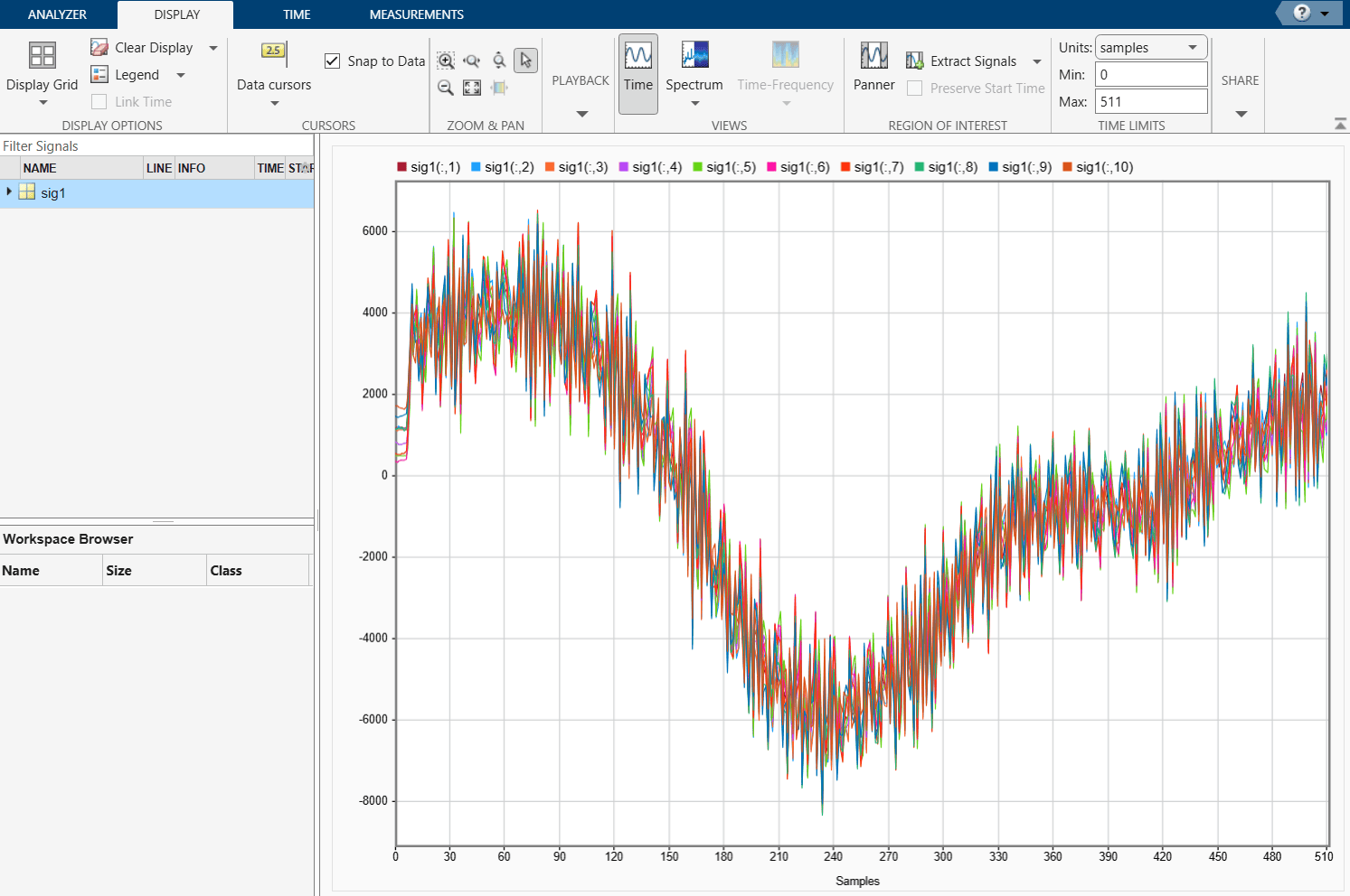
Display time samples from the first CPI.
signalAnalyzer(squeeze((data(1,:,:))))
Processing the Data
In this dataset, the drones are either hovering or rotating in place at a known distance, so no detection or tracking is performed here. If the drone were moving, an adaptive detector like phased.CFARDetector2D may be useful for detecting the drone. In this scenario when advanced detection techniques are not needed, isolating the drone micro-Doppler is implemented using the following steps for each CPI:
Perform the range FFT (The signal is already dechirped. See
dechirpfor more details).Sum the range bins that contain the drone along the range dimension.
Concatenate the summed range bins for each chirp.
% Isolate the range bins containing the drone
startRangeBin = floor(info.startRange/info.rangeRes);
endRangeBin   = ceil(info.endRange/info.rangeRes);

% Define a range processor
rangeProc = helperCreateProcessors(info);
nCPI      = size(data,1);
nChirps   = size(data,3);
cpiSums   = zeros(nCPI*nChirps,1); % Used to store relevant range bins

for cpiIdx = 1:size(data,1)
    cpi = squeeze(data(cpiIdx,:,:));
    [respR, rngGrid] = rangeProc(cpi);
    if isreal(cpi(1,1)) % If data is real, take positive spectrum only
        respR   = respR(1:round(numel(rngGrid)/2),:);
        rngGrid = rngGrid(1:round(numel(rngGrid)/2));
    end
    % Sum range bins that contain drone -> 1 complex value per chirp
    cpiSum   = sum(respR(startRangeBin:endRangeBin,:),1);
    pulseIdxs = ((cpiIdx-1)*nChirps:cpiIdx*nChirps-1)+1;
    cpiSums(pulseIdxs) = cpiSum;
end
HERM Lines
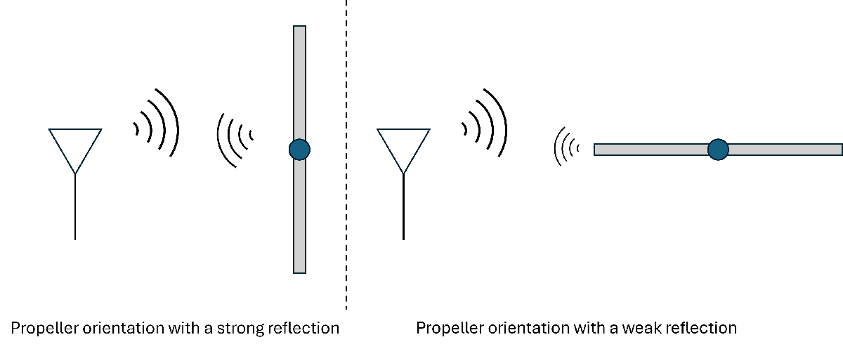
Drones and helicopters have micro-Doppler signatures characterized by HERM lines, or HElicopter Rotor Modulation lines, caused by the rotating propellers. These signatures result from the changing radar cross section arising from the orientation of the spinning blades. As shown in the graphic above, when a rotor blade is perpendicular to the propagating radar signal, the reflected energy is high. In contrast, when the blade is parallel to the propagating signal, the reflected energy is low. This fluctuation in received power is captured in the micro-Doppler information and appears as lines when the observation time is sufficient. To capture these fluctuations, the dwell time on the target with propellers must be longer than one full rotation of the blades. In addition, HERM lines are more apparent when multiple revolutions are observed. In other words, longer dwell times lead to more pronounced HERM lines.
Given a rotation period of and blades, the fundamental frequency of the observed Doppler is [5]. This frequency is observed as a Doppler shift about the operating frequency. Strong harmonics also appear at integer multiples of the fundamental frequency. Visualize the HERM lines for the recordings contained in droneDS by taking the short-time Fourier transform (STFT) of the summed range bins from each chirp. Notice how the HERM lines become more visible as the window length increases.
fig   = figure;
tl    = tiledlayout(3,1);
ax    = gobjects(1,3);
axIdx = 1;

for windowLen = 2.^([4 7 9])
    ax(axIdx) = nexttile;
    axIdx   = axIdx + 1;
    win     = kaiser(windowLen,6);
    [s,f,t] = stft(cpiSums,1/info.pri,"FFTLength",1024,Window=win,OverlapLength=windowLen/2);
    sPower  = mag2db(abs(s).^2);

    if strcmpi(radarFrequency,'94GHz')
        % The negative sign is due to how the mixer was implemented in the 94 GHz radar
        f = -f;
    end

    imagesc(t,f,sPower)
    colormap("jet")
    clim([prctile(sPower(:),10),max(sPower(:))])
    title(['Window length of ',num2str(windowLen)])
    xlabel('Time (s)')
    ylabel('Doppler (Hz)')
end

title(tl,[info.droneModel ': ', info.flightPattern],'Interpreter', 'none')
linkaxes(ax, 'xy');  % Link all x-axes after the loop
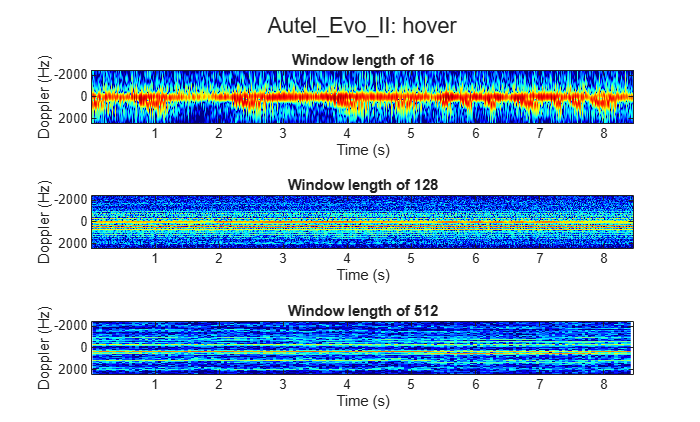
In the figures above, the strong reflection at 0 Hz is from the drone body. The parallel lines above and below the body are the HERM lines arising from rotor blade reflections. To visualize the HERM lines more clearly and to see how prominent each frequency is throughout each recording, use pspectrum. For recordings with a rotating drone, this helps to visualize the different engine speeds used to rotate and stabilize the drone.
You will plot two key metrics to identify different drone models and behaviors. First, you will plot the chopping frequency, which measures how often the rotating blades cross the radar beam to create blade flashes. Next, you will plot the spool frequency to show the actual rotation per minute (rpm) of the drone’s motor and shaft.
% Parameters
frequencyLimits = sort([f(1) f(end)]);
overlapPercent  = 50;

% Compute spectral estimate
% Run the function call below without output arguments to plot the results
figure;
pspectrum(cpiSums, 1/info.pri, ...
    'persistence', ...
    'FrequencyLimits',frequencyLimits, ...
    'OverlapPercent',overlapPercent,'TimeResolution',1);
hold on

% Add HERM lines.
% Need to Update the plotted fundamental frequency for different drone types or activities
fundamentalFrequency = 166; %Hz

% Fundamental frequency line
hermFundamentalFrequencyLine = fundamentalFrequency/1e3;
xline(hermFundamentalFrequencyLine,'--',Color='red',LineWidth=2,DisplayName='Fundamental frequency')

% Chopping frequency lines - only first visible to legend
hermChoppingLines = [-4:-1 2:4]*fundamentalFrequency/1e3;
xline(hermChoppingLines(1),'-.',Color='yellow',LineWidth=2,DisplayName='Chopping line')
xline(hermChoppingLines(2:end),'-.',Color='yellow',LineWidth=2,HandleVisibility='off')

% Spool frequency lines - only first visible to legend
hermSpoolLines = fundamentalFrequency/2e3 + (-4:3)*fundamentalFrequency/1e3;
xline(hermSpoolLines(1),':',Color='magenta',LineWidth=2,DisplayName='Spool line')
xline(hermSpoolLines(2:end),':',Color='magenta',LineWidth=2,HandleVisibility='off')

xlim([-0.6 0.6])
lgd = legend('Location','northwest');
title(lgd, 'HERM Line Components')
fontsize(lgd, scale=0.8);
hold off
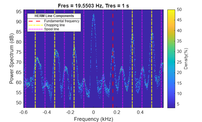
Notice the first strong harmonic for the hovering Autel Evo II is around 0.166 kHz. Because the propellers have two blades for each motor, we can determine that each motor is spinning at 0.083 kHz, which is equivalent to a motor operating at 4980 rpm. For the cases where the drones perform other maneuvers than just hovering, the persistence spectrum will display rotor speed at different fundamental frequencies along with their harmonics. Next, you will investigate the data transformation for the bird data and see how the bird micro-Doppler differs from the drones' micro-Doppler.
Bird Data
Create a signalDatastore for the bird data using the same custom read function from the drone datastore.
parentDir = ['.' filesep fileName filesep];
folder    = ['bird' radarFrequency];
birdDS    = signalDatastore(fullfile(parentDir,folder),ReadFcn=@helperCustomreader);
Just like with the drone data, there is also important metadata associated with each recording such as the bird species and comments about its flight pattern. The range resolution is in meters; the operating frequency is in Hz; the PRI is in seconds.
if hasdata(birdDS)
    [data,info] = read(birdDS);
    info = rmfield(info,"FileName")
end
info = struct with fields:
                  bird: 'Bald Eagle'
              comments: '10-24-42 to 12-24-50 fly from 80m to 40m. 3-11'
      nSamplesPerChirp: 512
    operatingFrequency: 2.4000e+10
                   pri: 2.0000e-04
              rangeRes: 0.6000
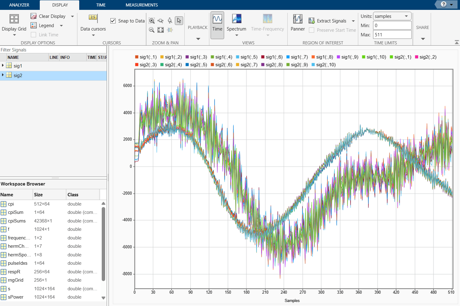
Add time samples from the first CPI of the bird dataset to the signalAnalyzer plot, which already contains time samples from the first CPI of the drone dataset.
signalAnalyzer(squeeze((data(1,:,:))))
Detecting the Bird
In contrast to the drone data, the recorded bird data contains birds flying between two points, such as benches, falconers, or the ground. Clutter suppression and moving target detection can help to isolate the reflections from the bird, making the micro-Doppler easier to see and analyze.
To save processing time, use the knowledge that the birds flew at ranges between 20 and 85 meters for all the recording. This will cut down the search space for the bird.
% Bird flew between 20 and 85 meters
startRangeBin  = floor(20/info.rangeRes);
endRangeBin    = ceil(85/info.rangeRes);
tgtRangeBinOld = round((startRangeBin+endRangeBin)/2); % Used for initialization when no bird is detected
Define a constant false alarm rate (CFAR) detector using phased.CFARDetector2D. Make sure to allow for detections near the maximum unambiguous Doppler-velocities by circular padding the Doppler dimension.
[detector,cutIdx] = helperSetupCFAR(size(data,3),startRangeBin,endRangeBin);
Construct range and range-Doppler processors. The range-Doppler processor will be used to detect the bird while the range-Response will be used as input to the STFT that visualizes the micro-Doppler for the duration of the recording.
[rangeProc,rangeDopProc] = helperCreateProcessors(info);
cpiSums = [];
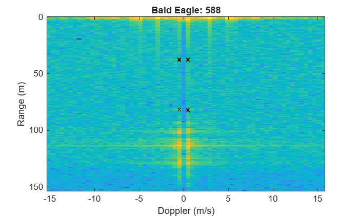
Iterate through each recording and output the sum of the relevant range bins for each chirp just as you did with the drone data. Also, visualize the range-Doppler response and the associated detections for each CPI.
figure

for cpiIdx = 1:size(data,1)
    cpi = squeeze(data(cpiIdx,:,:));
    cpi = cpi - mean(cpi,2); % Suppress static clutter
    [respRD,rngGrid,dopGrid] = rangeDopProc(cpi);
    respR = rangeProc(cpi);
    if isreal(cpi(1,1)) % If data is real, take positive spectrum only
        respR   = respR(1:round(numel(rngGrid)/2),:);
        respRD  = respRD(1:round(numel(rngGrid)/2),:);
        rngGrid = rngGrid(1:round(numel(rngGrid)/2));
    end
    respPow = abs(respRD).^2;

    if cpiIdx == 1 % Set up plot
        axImage = imagesc(dopGrid,rngGrid,pow2db(respPow));
        xlabel('Doppler (m/s)')
        ylabel('Range (m)')
        hold on
        axDets = plot(nan,nan,'kx');
    else
        axImage.CData = pow2db(respPow);
    end
    title([info.bird, ': ', num2str(cpiIdx)])

    % Get detections
    dets = detector(respPow,cutIdx,20);
    detLocs = cutIdx(:,dets);
    if ~isempty(detLocs)
        tgtRangeBin = unique(detLocs(1,:));
        axDets.XData = dopGrid(detLocs(2,:));
        axDets.YData = rngGrid(detLocs(1,:));
        tgtRangeBinOld = tgtRangeBin;
        cpiSum = sum(respR(tgtRangeBin,:),1);
        cpiSums = [cpiSums cpiSum]; %#ok
    end

    pause(.01) % For visualization
end
Visualize the bird's micro-Doppler using the STFT just as with the drone data.
fig = figure;
tl  = tiledlayout(3,1);
ax  = gobjects(1,3);
axIdx = 1;

for windowLen = 2.^([4 7 9])
    ax(axIdx) = nexttile;
    axIdx = axIdx + 1;
    win   = kaiser(windowLen,6);
    [s,f,t] = stft(cpiSums,1/info.pri,"FFTLength",1024,Window=win,OverlapLength=windowLen/2);
    sPower  = mag2db(abs(s).^2);

    if strcmpi(radarFrequency,'94GHz')
        % The negative sign is due to how the mixer was implemented in the 94 GHz radar
        f = -f;
    end

    % You should account for two-way doppler shift when converting
    % doppler frequency to speed
    dop = dop2speed(f,freq2wavelen(info.operatingFrequency))/2;
    imagesc(t,dop,sPower)
    colormap("jet")
    clim([prctile(sPower(:),40),max(sPower(:))])
    title(['Window length of ',num2str(windowLen)])
    xlabel('Time (s)')
    ylabel('Doppler (m/s)')
end

title(tl,info.bird)
linkaxes(ax, 'xy');  % Link all x-axes after the loop
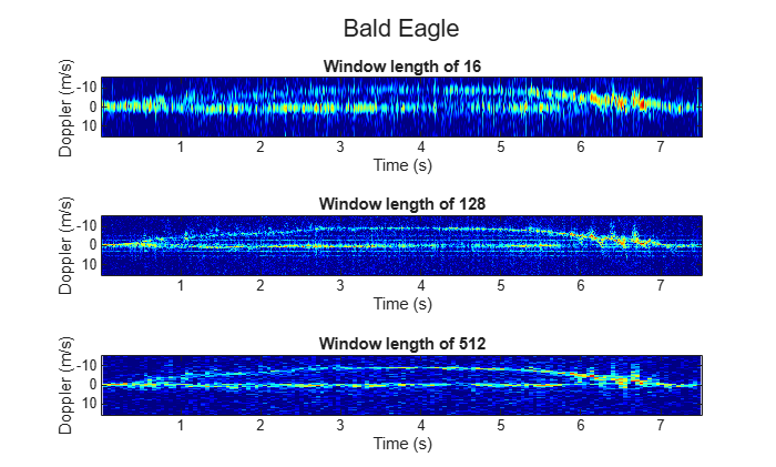
You can make several observations from the bird data. First, notice the strong returns from the falconer near 0 m/s. Next, notice how the bird speeds up to roughly 9 m/s and then slows down. During the segments of acceleration, you can see Doppler-signatures from the bird's flapping wings. When the bird is not accelerating as much, the bird resembles much more of a point target.
Each radar has its own artifacts that are also worth mentioning. In the range-Doppler map of the 24 GHz data, you can see very strong range sidelobes from very close scatterers. These reflections also appear in the spectrogram and should not be confused with HERM lines. In the 94 GHz data, first notice that the Doppler values are the opposite of that of the 24 GHz data. This is because of mixer implementation as described in an earlier section. Finally, some micro-Doppler plots from the bird dataset may show no detectable signal for a short period because the bird flew outside the radar's main beam.
Classifying Micro-Doppler with a Neural Network
Target identification is an important task in many radar applications. We demonstrate the ability to distinguish between bird and drone micro-Doppler by creating a dataset of processed micro-Doppler data and then using a neural network to classify the signatures. Both the drone data and the bird data were processed identically except for how the detection was performed. Just as above we used the known range information to isolate the drones and we used CFAR to isolate the birds. The processing pipeline is portrayed in the figure below.

The STFT has a window length of 12.5 ms and 512 Doppler bins. Both datasets split the recording into matrices that contain 1 second of data where each column is one processing window of the STFT. That means that each input is of the size 512 by 80 meaning there are 80 windows, each with 512 Doppler bins. The results were then squared to convert to power values and then converted to decibels.
Download the micro-Doppler dataset before post processing the data and training the neural network
outputFolder         = pwd;
radarSupportfilesURL = 'https://ssd.mathworks.com/supportfiles/radar/data/';
fileNameNN           = 'droneBirdSpectrogramDataset';
helperDownloadDataset(outputFolder,radarSupportfilesURL,fileNameNN);
Augmenting the dataset
In deep learning, adding random transformations to the data can reduce the amount of overfitting. This is especially necessary when the dataset is small, as in this case. For a signalDatastore, the easiest way to perform such augmentations is to apply them in a new custom read function just as was done above.
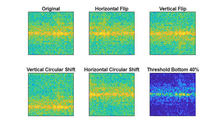
Construct a signal datastore with a custom read function that performs the following transforms:
Transformation | Motivation |
Random Horizontal Flips | This acts as a time reversal (horizontal dimension is time). |
Random Vertical Flips | This negates the Doppler information. This is especially useful since the 94 GHz radar has a negated Doppler return as explained above. |
Random Vertical Circular Shifts | This simulates a uniform Doppler shift of the data. One interpretation of this is adding ego-velocity to the radar without range migration. |
Random Horizontal Circular Shifts | This simulates is a circular shift in time. |
Threshold the Noise Floor | This reduces the dynamic range of the data. Thresholding here instead of during the creation of the dataset allows for easy prototyping during training. |
View each transform on the same image below.
rng('default');

testInput = load(['.' filesep fileNameNN filesep 'drone' filesep 'Yuneec_H520E_rotate__12_24GHz.mat']).matOut;
helperShowTransforms(testInput)
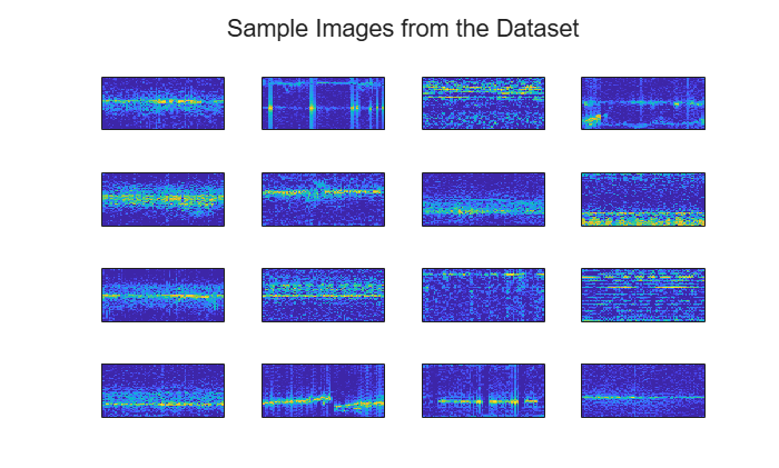
Preview the full dataset with the random transforms specified above.
nnDS = signalDatastore(['.' filesep fileNameNN],IncludeSubfolders=true, ...
    ReadFcn=@helperDLreader,FileExtensions='.mat');
shuffledNnDS = shuffle(nnDS);

figure;
sampleTL = tiledlayout(4,4);

for ii = 1:16
    nexttile
    data = read(shuffledNnDS);
    imagesc(data);
    set(gca,'xtick',[])
    set(gca,'ytick',[])
end

title(sampleTL,'Sample Images from the Dataset')
Create labels for each input based on the directory containing the data using an arrayDatastore. Then, combine the datastores that contain the inputs and their labels.
labels = folders2labels(nnDS);
nnDS = combine(nnDS, arrayDatastore(labels));
Display the number of inputs for each class.
cats   = categories(labels);
counts = countcats(labels);

for ii = 1:2
    fprintf('There are %d inputs of category %s\n',counts(ii),cats{ii})
end
There are 126 inputs of category bird
There are 346 inputs of category drone
Next, split the dataset into training and test datasets. Use 80% for training and the rest for testing. Due to the small size of the dataset, use the test dataset for validation during training.
splitIndices = splitlabels(nnDS,0.8,UnderlyingDatastoreIndex=2);
trainDS = subset(nnDS,splitIndices{1});
testDS = subset(nnDS,splitIndices{2});
Create a Lightweight Neural Network
While MATLAB does have many pretrained networks (Built-In Pretrained Networks (Deep Learning Toolbox)), many of them impose restrictions on the input size and pixel values. To circumvent these constraints and to achieve an even lighter weight network then the pretrained models, construct a new neural network that is only a few layers deep. This is quite reasonable given the simplicity of the task, i.e. binary classification. Because the aspect ratio of the inputs is very tall 32:5 and the micro-Doppler features like HERM lines span many Doppler bins, it is important to create a network with filters that are big enough to detect said features. To accomplish this, make sure that the network has tall (not square) filters and that the pooling layers downsample the vertical dimension faster than the horizontal dimension so that the filters can get progressively smaller for each successive layer.
imageSize  = size(data);
numClasses = 2;
layers = [
    imageInputLayer(imageSize,"Normalization","rescale-symmetric")

    convolution2dLayer([7 5],8,Padding="same")
    batchNormalizationLayer
    reluLayer
    maxPooling2dLayer([4 2],Stride=[4 2])

    convolution2dLayer([5 3],16,Padding="same")
    batchNormalizationLayer
    reluLayer
    maxPooling2dLayer([4 2],Stride=[4 2])

    convolution2dLayer([3 3],32,Padding="same")
    batchNormalizationLayer
    reluLayer
    dropoutLayer(.4)

    fullyConnectedLayer(numClasses)
    softmaxLayer];

% Visualize the network architecture
networkInfo = analyzeNetwork(layers,Plots="none");
networkInfo.LayerInfo
ans = 15×7 table
Name Type ActivationSizes ActivationFormats LearnableSizes NumLearnables StateSizes
_____________ _____________________ _______________ _________________ ______________________________________________ _____________ ______________________________________________
"imageinput" "Image Input" {[ 512 80 1 1]} {["SSCB"]} {[dictionary (string ⟼ cell) with no entries]} 0 {[dictionary (string ⟼ cell) with no entries]}
"conv_1" "2-D Convolution" {[ 512 80 8 1]} {["SSCB"]} {[dictionary (string ⟼ cell) with 2 entries ]} 288 {[dictionary (string ⟼ cell) with no entries]}
"batchnorm_1" "Batch Normalization" {[ 512 80 8 1]} {["SSCB"]} {[dictionary (string ⟼ cell) with 2 entries ]} 16 {[dictionary (string ⟼ cell) with 2 entries ]}
"relu_1" "ReLU" {[ 512 80 8 1]} {["SSCB"]} {[dictionary (string ⟼ cell) with no entries]} 0 {[dictionary (string ⟼ cell) with no entries]}
"maxpool_1" "2-D Max Pooling" {[ 128 40 8 1]} {["SSCB"]} {[dictionary (string ⟼ cell) with no entries]} 0 {[dictionary (string ⟼ cell) with no entries]}
"conv_2" "2-D Convolution" {[128 40 16 1]} {["SSCB"]} {[dictionary (string ⟼ cell) with 2 entries ]} 1936 {[dictionary (string ⟼ cell) with no entries]}
"batchnorm_2" "Batch Normalization" {[128 40 16 1]} {["SSCB"]} {[dictionary (string ⟼ cell) with 2 entries ]} 32 {[dictionary (string ⟼ cell) with 2 entries ]}
"relu_2" "ReLU" {[128 40 16 1]} {["SSCB"]} {[dictionary (string ⟼ cell) with no entries]} 0 {[dictionary (string ⟼ cell) with no entries]}
"maxpool_2" "2-D Max Pooling" {[ 32 20 16 1]} {["SSCB"]} {[dictionary (string ⟼ cell) with no entries]} 0 {[dictionary (string ⟼ cell) with no entries]}
"conv_3" "2-D Convolution" {[ 32 20 32 1]} {["SSCB"]} {[dictionary (string ⟼ cell) with 2 entries ]} 4640 {[dictionary (string ⟼ cell) with no entries]}
"batchnorm_3" "Batch Normalization" {[ 32 20 32 1]} {["SSCB"]} {[dictionary (string ⟼ cell) with 2 entries ]} 64 {[dictionary (string ⟼ cell) with 2 entries ]}
"relu_3" "ReLU" {[ 32 20 32 1]} {["SSCB"]} {[dictionary (string ⟼ cell) with no entries]} 0 {[dictionary (string ⟼ cell) with no entries]}
"dropout" "Dropout" {[ 32 20 32 1]} {["SSCB"]} {[dictionary (string ⟼ cell) with no entries]} 0 {[dictionary (string ⟼ cell) with no entries]}
"fc" "Fully Connected" {[ 2 1]} {["CB" ]} {[dictionary (string ⟼ cell) with 2 entries ]} 40962 {[dictionary (string ⟼ cell) with no entries]}
"softmax" "Softmax" {[ 2 1]} {["CB" ]} {[dictionary (string ⟼ cell) with no entries]} 0 {[dictionary (string ⟼ cell) with no entries]}
Get insights using Copilot
Train the Neural Network
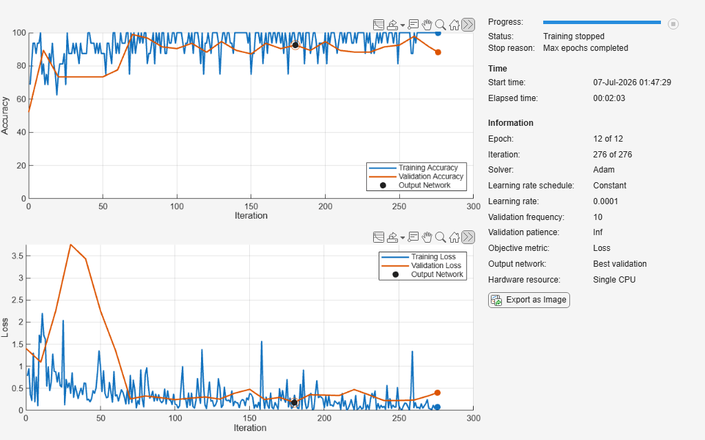
Define the training parameters and train the network. During training, make sure to save the best performing set of weights and not just the last by adding the name-value pair, OutputNetwork="best-validation". Note that this network converges rapidly because there are so few learnable parameters and the task is relatively simple.
options = trainingOptions("adam", ...
    MaxEpochs          = 12, ...
    Metrics            = "accuracy", ...
    ValidationData     = testDS, ...
    ValidationFrequency= 10, ...
    MiniBatchSize      = 16, ...
    Verbose            = false, ...
    InitialLearnRate   = 1e-4,...
    Shuffle            = "every-epoch",...
    Plots              = "training-progress",...
    OutputNetwork      = "best-validation");
Because this dataset is unbalanced, i.e. many more drone inputs than bird inputs, create a custom loss function that penalizes the network more for the bird inputs.
frequency    = counts/sum(counts);
classWeights = dlarray(1 ./ frequency,"C");
lossFcn      = @(Y,T)crossentropy(Y,T,classWeights);
Train the network.
net = trainnet(trainDS,layers,lossFcn,options);
Test the Neural Network
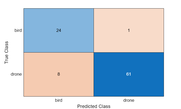
Now that the neural network is trained, compute the test dataset classification accuracy and display the associated confusion matrix. The confusion matrix shows how many inputs of each class were properly and improperly classified.
YTest = minibatchpredict(net,testDS);
YTest = scores2label(YTest,cats);

% Evaluate the classification accuracy for the test data. The accuracy is the percentage of correct predictions.
TrueTest = readall(testDS.UnderlyingDatastores{2});
TrueTest = string([TrueTest{:}]);
accuracy = mean(TrueTest'==string(YTest))
accuracy = 0.9043
figure;
confusionchart(TrueTest,string(YTest))
Finally, visualize which micro-Doppler features the neural network uses to distinguish between birds and drones using gradCAM. gradCAM utilizes the gradients of the classification score with respect to the final convolutional feature map, to identify the parts of an input image that most impact the classification score.
fig               = figure;
fig.Position(3:4) = [1920 1000];
testDS            = shuffle(testDS);

tiledlayout(2,8,'TileIndexing','columnmajor')
for ii = 1:8
    data       = read(testDS);
    inputData  = data{1};
    labelTruth = data{2};
    scores     = predict(net,inputData);
    [labelPred,score] = scores2label(scores,cats);

    nexttile
    imagesc(inputData)
    set(gca,'xtick',[])
    set(gca,'ytick',[])
    title({"Pred: " + string(labelPred), ...
        "Truth: " + string(labelTruth)})

    % Show Location of Interest for Prediction
    scoreMap = gradCAM(net,inputData,labelPred);

    nexttile
    imagesc(scoreMap)
    set(gca,'xtick',[])
    set(gca,'ytick',[])
    colormap jet;
    title('Grad-CAM')
end
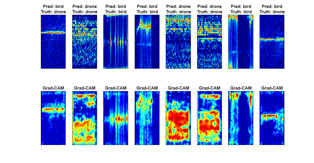
From the images above, notice how the network uses the strongest returns from the bird while it uses the higher order harmonics of the drone to classify the inputs.
Summary
This example presents a novel dataset that captures the micro-Doppler signatures of five drones and five birds, each with two different FMCW radars. You saw how to organize datasets into datastores for easy loading and manipulation of large amounts of data. You then explored the dataset and observed micro-Doppler features such as drone HERM lines and bird wings flapping. Finally, you distinguished between bird and drone micro-Doppler by creating and augmenting a dataset of processed micro-Doppler data and then trained a lightweight neural network to classify their signatures.
References
[1] Z. Guo, "MathWorks Radar Drone Project," GitHub, 2025. Accessed: Jun. 23, 2026. [Online]. Available: https://github.com/ZhongliangGuo/MathWorks-Radar-Drone-Project/tree/main
[2] S. Rahman and D. A. Robertson, "Radar micro-Doppler signatures of drones and birds at K-band and W-band," Sci. Rep., vol. 8, art. 17396, 2018.
[3] S. Rahman and D. A. Robertson, "Coherent 24 GHz FMCW radar system for micro-Doppler studies," in Proc. Radar Sensor Technology XXII, vol. 10633, pp. 154–162, SPIE, 2018.
[4] D. A. Robertson, G. M. Brooker, and P. D. L. Beasley, "Very low-phase noise, coherent 94 GHz radar for micro-Doppler and vibrometry studies," in Proc. Radar Sensor Technology XVIII, vol. 9077, SPIE, 2014.
[5] D. Blacknell and H. Griffiths, Radar Automatic Target Recognition (ATR) and Non-Cooperative Target Recognition (NCTR), no. 11300. IET, 2013.
Helper Functions
function helperDownloadDataset(outputFolder,radarSupportfilesURL,fileName)
% Download the dataset from the given URL to the output folder.

radarDataFile = fullfile(outputFolder,fileName);

if ~exist(radarDataFile,'file')

    extension = '.zip';
    disp(['Downloading the large dataset file ''',fileName, extension, '''. Might take multiple minutes to finish downloading ...']);
    dataURL = [radarSupportfilesURL,fileName,extension];
    websave(radarDataFile,dataURL);

    unzip(radarDataFile,fullfile([outputFolder filesep fileName]));
end
end
function [data,info] = helperCustomreader(filename)
% Custom read function for loading the drone and bird raw data

matFile   = load(filename);
fieldList = fieldnames(matFile);

for field = fieldList'
    field = field{1}; %#ok
    if strcmpi(field,'cpis')
        data = matFile.(field);
    else
        info.(field) = matFile.(field);
    end
end
end
function [rangeProc, rangeDopProc] = helperCreateProcessors(info)
% Define range and range-Doppler processors

fs         = info.nSamplesPerChirp/info.pri;
bandWidth  = physconst('LightSpeed')/2/info.rangeRes;
sweepSlope = bandWidth/info.pri;

rangeDopProc = phased.RangeDopplerResponse(...
    RangeMethod            = 'FFT',...
    DechirpInput           = false, ...
    ReferenceRangeCentered = false,...
    SweepSlope             = sweepSlope,...
    SampleRate             = fs,...
    RangeWindow            = 'Taylor',...
    DopplerWindow          = 'Kaiser',...
    OperatingFrequency     = info.operatingFrequency,...
    DopplerOutput          = 'Speed');

rangeProc = phased.RangeResponse(...
    RangeMethod            = 'FFT',...
    DechirpInput           = false, ...
    ReferenceRangeCentered = false,...
    SweepSlope             = sweepSlope,...
    SampleRate             = fs,...
    RangeWindow            = 'Taylor');
end
function [detector,cutIdx] = helperSetupCFAR(nChirps,rBinStart,rBinEnd)
% Define CFAR detector

detector = phased.CFARDetector2D( ...
    'TrainingBandSize',[5,3], ...
    'ThresholdFactor','Input port', ...
    'GuardBandSize',[5,3], ...
    'Method','CA');
Ngc = detector.GuardBandSize(2);
Ntc = detector.TrainingBandSize(2);

cutIdx   = [];
colstart = Ntc + Ngc + 1;
colend   = nChirps - ( Ntc + Ngc);
rowstart = rBinStart;
rowend   = rBinEnd;

for m = colstart:colend
    for n = rowstart:rowend
        cutIdx = [cutIdx,[n;m]]; %#ok
    end
end
end
function data = helperDLreader(filename)
% Custom read function that transforms the data for training the neural network

a = load(filename);
data = a.matOut;
if rand() > 0.5
    data = flipud(data);
end
if rand() > 0.5
    data = fliplr(data);
end

maxShift = round(.3 * size(data,1));
data = circshift(data,randi(maxShift*[-1,1]),1);

maxShift = round(.5 * size(data,2));
data = circshift(data,randi(maxShift*[-1,1]),2);

% constrains the dynamic range
bottom40 = prctile(data,40,"all");
data(data<bottom40) = bottom40;
end
function helperShowTransforms(testInput)
% Helper plotting function

figure
tiledlayout(2,3)

nexttile
imagesc(testInput)
set(gca,'xtick',[])
set(gca,'ytick',[])
title('Original')

nexttile
imagesc(fliplr(testInput))
set(gca,'xtick',[])
set(gca,'ytick',[])
title('Horizontal Flip')

nexttile
imagesc(flipud(testInput))
set(gca,'xtick',[])
set(gca,'ytick',[])
title('Vertical Flip')

nexttile
imagesc(circshift(testInput,150,1))
set(gca,'xtick',[])
set(gca,'ytick',[])
title('Vertical Circular Shift')

nexttile
imagesc(circshift(testInput,30,2))
set(gca,'xtick',[])
set(gca,'ytick',[])
title('Horizontal Circular Shift')

nexttile
bottom40 = prctile(testInput,40,"all");
testInput(testInput<bottom40) = bottom40;
imagesc(testInput)
set(gca,'xtick',[])
set(gca,'ytick',[])
title('Threshold Bottom 40%')
end
See Also
convolution2dLayer (Deep Learning Toolbox) | signalDatastore

