Scan Dosing Regimens Using SimBiology Model Analyzer App

This example shows how to assess the efficacy and toxicity of various dose amounts in the SimBiology Model Analyzer app by using the target (receptor) occupancy as a biomarker. The example uses the target-mediated drug disposition (TMDD) model [1] with slight modifications.

Target-Mediated Drug Disposition (TMDD) Model

Target-mediated drug disposition (TMDD) is a phenomenon in which a drug binds with high affinity to its pharmacologic target site, such as a receptor or enzyme, in an interaction that is reflected in the pharmacokinetic characteristics of the drug.

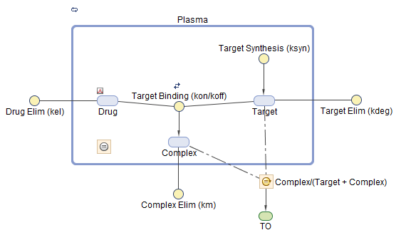
This example uses a modified TMDD model based on the model used by Mager and Jusko [1] with a minor adjustment. The authors proposed a generic TMDD model that accounted for saturable drug-target binding and target (or receptor) mediated elimination. Drug in the Plasma reversibly binds with the unbound Target to form the drug-target Complex. kon and koff are the association and dissociation rate constants, respectively. Clearance of free Drug and Complex from the Plasma is described by first-order processes with rate constants — kel and km, respectively. Free target turnover is described by the zero-order synthesis rate ksyn and a first-order elimination (the rate constant, kdeg). Variants of the TMDD model have been since used to characterize the pharmacokinetics of numerous drugs.

One adjustment made to the model presented by Mager and Jusko, is as follows.

Target occupancy (TO) is defined as TO = Complex/(Target + Complex), where TO is a parameter and Complex and Target are species.

Load TMDD Model

Enter the following command. SimBIology Model Analyzer opens. In the Browser pane, the Models folder contains the TMDD model.

openExample('simbio/ScanDosesSimBiologyModelAnalyzerExample')

Generate Array of Doses and Simulate Model

First, create a program to generate an array of doses with different dose amounts ranging from 0 to 300 nanomoles.

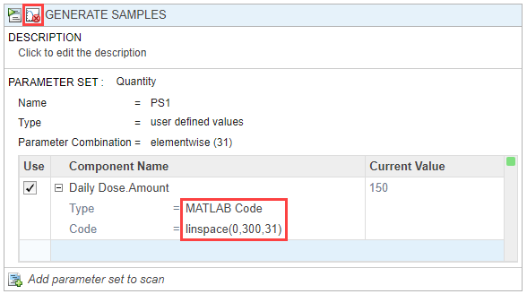
Select Program > Generate Samples. In the Generate Samples step, double-click the empty cell under Component Name and enter Daily Dose.Amount.

Under Daily Dose.Amount, set Type to MATLAB Code, and set Code to linspace(0,300,31). This code specifies the generation of 31 doses with amounts ranging from 0 to 300 nanomoles.

Disable the plotting of dose samples by clicking the plot button, as shown in the figure.

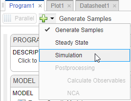
Add a simulation step to simulate the model using the defined doses. Click the (+) icon at the upper left of the program and select Simulation. A Simulation step appears following the Generate Samples step.

In the Model step, click States to Log. Select TO as the only state to log by clearing all other check boxes.

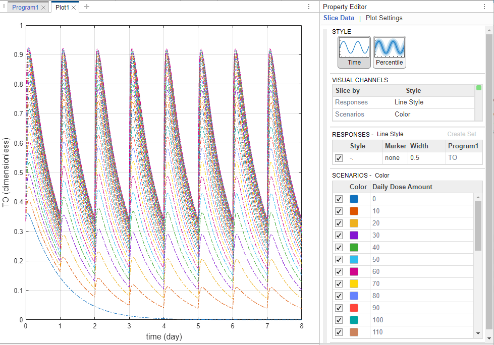
On the Home tab, click Run. Once the simulation is complete, the program plots the results in Plot1, which shows the time course of the model response (TO) given different dose amounts.

Tip: Plots are backed by data that are currently present in the app workspace. Plots are not snapshots. When the data (either experimental data or simulation results) is removed or changed, the plots are also updated according to the changes in the underlying data.

Define Maximum and Minimum Target Occupancy Thresholds

Investigate which dose amounts correspond to the TO responses that lie within the safety (TO = 0.85) and efficacy (TO = 0.15) thresholds. One approach is to add two (horizontal) threshold lines to the TO response plot.

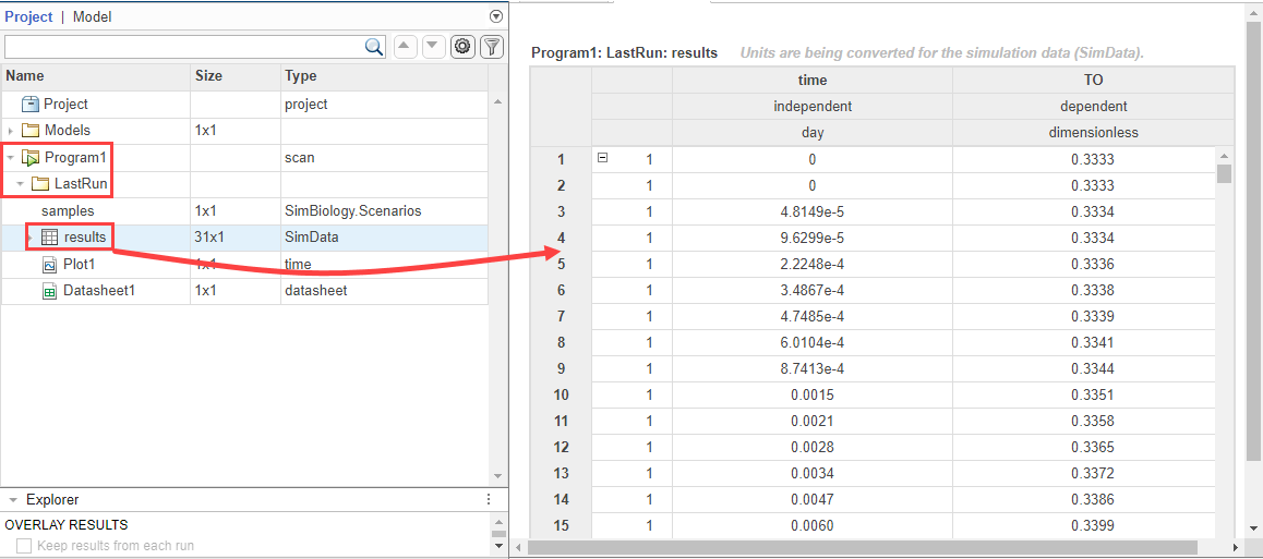
On the Home tab, in the Project section, click New Datasheet. In the Browser pane, expand the Program1 folder, then expand the LastRun folder.

Drag results into the new datasheet. The datasheet now shows time and TO columns with their corresponding values.

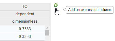
Point to the table and add an expression by clicking the (+) icon that appears at the top right.

Note: Anytime you add an expression to a datasheet containing results from LastRun, the expression is added as an observable object to the model. In addition, the Postprocessing: Calculate Observables step is also added to the corresponding program that generated the LastRun data.

Double-click Name1 and rename it EfficacyThreshold.

Double-click UNITS and enter dimensionless.

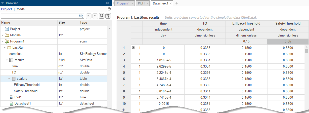
Double-click the Expression cell and enter 0.15. The expression fills the column with the same constant value (0.15) for every time point.

Similarly, add another expression column named SafetyThreshold with the expression 0.85. Expand results in the LastRun folder. The values from these two expression columns are scalar-valued observables and now stored in the table named scalars under results. You can now plot the maximum and minimum threshold lines on to the existing plot Plot1.

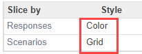
Click the Plot1 tab. Press Ctrl and select EfficacyThreshold and SafetyThreshold variables from the Browser pane. Drag them into the plot. The plot now shows TO profiles along with the efficacy and safety threshold lines.

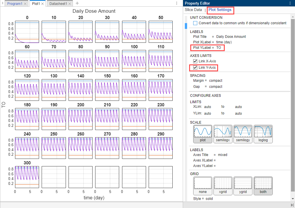
Visualize Target Occupancy Responses on Separate Axes

The plot shows that certain TO responses either exceed the safety threshold or dip below the efficacy threshold. To better visualize this observation, you can customize the plot to see each dose amount and the corresponding TO response on separate axes.

Click Plot Settings. For Plot YLabel, enter TO as the value. In the Axes Limits section, select Link Y-Axis to show the same set of labels on the y-axis for all subplots.

Postprocess Simulation Results

In addition to visually inspecting each response plot on separate axes, you can add a postprocessing step to query exactly which dose amounts stay within the thresholds.

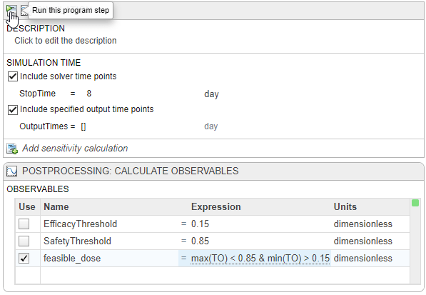
Click the Program1 tab. In the Postprocessing: Calculate Observables step, double-click the first empty cell in the Name column and enter: feasible_doses.

In the Expression column, enter max(TO) < 0.85 & min(TO) > 0.15. Set unit to dimensionless.

Note: Anytime you add an expression to the Observables table in the step, the expression is automatically added as an observable object to the corresponding model.

Select feasible_doses as the only observable. Clear EfficacyThreshold and SafetyThreshold. To evaluate feasible_doses, run just the simulation step by clicking the run button at the top of the Simulation step.

Running the program step generates the following figure. You might see a warning about dimensional analysis not being able to performed. For the purposes of this example, you can ignore the warning.

Display both the x-grid and y-grid by clicking both in the Grid section. The x-axis represents the dose amounts and the y-axis represents whether the dose amount generates a TO response that stays within the safety and efficacy thresholds (with a value of 1) or not (with a value of 0).

The plot shows that dose amounts ranging from 50 to 180 nanomoles provide TO responses that lie within the desired efficacy and safety thresholds.

References

[1] Marger, D., and W. Jusko. 2001. General pharmacokinetic model for drugs exhibiting target-mediated drug disposition. Journal of Pharmacokinetics and Pharmacodynamics. 28: 507–532.