R2023a

New Features, Bug Fixes, Compatibility Considerations

Simscape Language

Domain Equations: Use equations in domain files

In previous releases, the equations section was allowed only in a component file. The purpose of this section is to establish the mathematical relationships between the variables, parameters, inputs, and outputs of the component, the simulation time, and the time derivatives of each of these entities.

Now you can also include the equations section in a domain file, to establish the mathematical relationships between the domain Across variables, parameters, and intermediates. Domain equations propagate to the nodes of the corresponding domain type. Like the regular component equations, domain equations are executed throughout the simulation. You can also specify initial domain equations, similar to the initial component equations, to be executed during model initialization only.

For more information, see Domain Equations.

Scattered Lookup: Perform linear interpolation on a scattered set of data points

Use the scatteredlookup function in the equations section to compute an output value by interpolating the query input value against an unstructured, or scattered, set of data points. Unlike the tablelookup function, these data points do not need to form a table grid. You provide the coordinates of a set of input data points and the function value at each of these data points. Then you provide the coordinates of a query point or points and the scatteredlookup function returns the corresponding interpolated function value by using Delaunay triangulation.

The scatteredlookup function supports two-dimensional and three-dimensional lookup.

For more information, see scatteredlookup.

Functions for Arrays of Components and Nodes: Use array manipulation and query functions on an object array

Simscape™ language now allows you to use certain MATLAB^® functions on arrays of components and nodes to concatenate and reshape these arrays without using for-loops. You can also query an object array size and then use that size in a parametric expression in this or another object array.

The supported functions are:

Array manipulation: repmat, cat, horzcat, vertcat, reshape, transpose. These functions perform manipulations on the input object array and return an object array.
Array query: size, numel, ndims. These functions query the size aspects of an object array and return a result of primitive data type. These functions can be evaluated only at compile time.

For more information, see Using MATLAB Functions with Arrays of Components and Nodes.

Foundation Library

Block Dialog Box Enhancement: Use autocomplete and evaluated values for workspace variables

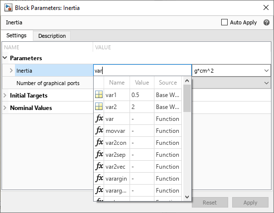
Simscape blocks now let you use autocomplete when you type in the block parameter fields. The autocomplete options include all the workspace variables in the current session.

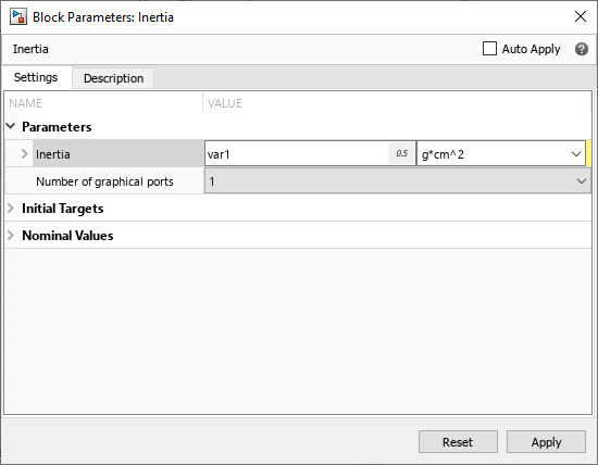
Block dialog box showing a list of autocomplete options

If you set a block parameter to a workspace variable or enter an expression, the block dialog box or Property Inspector evaluates the variable or expression and displays its current value in the parameter field.

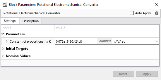
Block dialog box showing an evaluated variable

Block dialog box showing an evaluated expression

For more information, see View Values of Parameters Set as Variables.

PS Scattered Lookup Table (2D) and PS Scattered Lookup Table (3D) Blocks: Graphically define implicit equations that perform two-dimensional and three-dimensional scattered data lookup

The new PS Scattered Lookup Table (2D) and PS Scattered Lookup Table (3D) blocks in the Physical Signals/Lookup Tables library let you perform Delaunay triangulation on scattered sets of data points:

The PS Scattered Lookup Table (2D) block computes an approximation to some function f=f(x1,x2) given the coordinates of a set of input data points in a 2D space and function values at each of these data points. The two inputs and the output are physical signals.
The PS Scattered Lookup Table (3D) block computes an approximation to some function f=f(x1,x2,x3) given the coordinates of a set of input data points in a 3D space and function values at each of these data points. The three inputs and the output are physical signals.

For more information, see scatteredlookup.

Probe Enhancement: Select more variables to probe

The Probe block lets you select variables from another block in the model and output them as Simulink^® signals. In previous releases, when you selected the variables to output, the context menu contained only the variables exposed in the Initial Targets section of the block dialog box. These are the variables that you can use for block-level variable initialization.

Starting in R2023a, the context menu contains all the externally accessible block variables, regardless of whether they are exposed in the Initial Targets section of the block dialog box. Externally accessible variables include: block variables declared with the ExternalAccess attribute value of either modify or observe, inputs, outputs, intermediates, modecharts, and domain Across variables at each of the nodes. Essentially, these are the variables that you can see in the simulation data log.

To facilitate scanning through long lists of variables, especially in composite components, the display format of variables in the context menu has been reversed from Name:id to id:Name. For example, instead of Current:i, the same variable now appears as i:Current. This view is more consistent with the variable display in the Variable Viewer, Simscape Results Explorer, and Simulation Data Inspector.

The context menu now also has a filter field at the top. Type in this field to filter the variables displayed in the context menu.

Spectrum Analyzer Block: Use new toolstrip interface to visualize signals

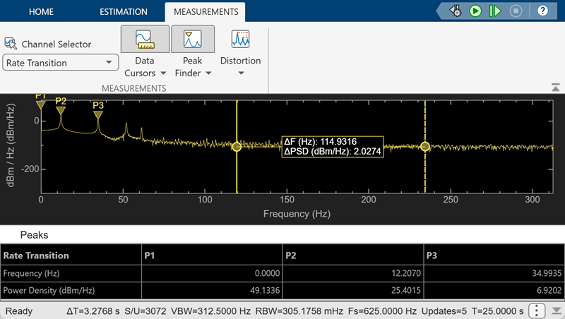
Use the improved Spectrum Analyzer block to visualize the frequency spectrum of the time-domain signals. The block is more responsive and has a new toolstrip interface that allows you easy access to spectral analysis, estimation, and measurement settings. You can configure and display Spectrum Analyzer settings from the command line with the SpectrumAnalyzerConfiguration object.

Frequency spectrum of signal in Spectrum Analyzer window

Rotational and Translational Hard Stop Enhancement: Use modeling option based on coefficient of restitution

The Rotational Hard Stop and Translational Hard Stop blocks have a new option for the Hard stop model parameter. This option, called Based on coefficient of restitution, models the hard stop by using a mode chart that includes free mode, where there is no torque or force transmission between the slider and the case, and static contact mode, where there is zero speed difference between the slider and the case. This modeling option improves simulation performance because static contact mode does not require the block to keep computing hard stop torque or force when the block is in contact mode.

Variable Thermal Mass Block: Vary thermal mass during simulation

In previous releases, thermal mass stayed constant during simulation. Now, the Thermal Mass block has a new parameter, Mass type:

Constant — The thermal mass is constant during simulation. This option is equivalent to how the block functioned in previous releases.
Variable — The thermal mass can vary during simulation. If you select this option, the Mass parameter in the block dialog is replaced by the Minimum mass parameter and a high-priority Mass variable, and the block has two physical signal input ports: Mdot, which specifies the change in the thermal mass, and Tin, which specifies the temperature of incoming mass. The signal value at port Tin has no effect when the thermal mass is constant or decreasing.

Use the Variable option to model systems where the mass changes but the geometric effects remain negligible, such as a washing machine being filled, heated, and then emptied with a varying amount of liquid per cycle.

Thermal Liquid Pressure and Flow Rate Sources That Perform No Thermodynamic Work: Configure flow conditions without affecting temperature

All blocks in the Thermal Liquid > Sources library have a new Power added parameter that lets you select whether the source performs work on the fluid flow:

Isentropic power — The source performs isentropic work on the fluid to maintain the specified pressure differential, mass flow rate, or volumetric flow rate depending on the source type. This is the default option, which is equivalent to the block behavior in previous releases. Use this option to represent an idealized pump or compressor and account for the energy input and output, especially in closed-loop systems.
None — The source performs no work on the flow, neither adding nor removing power, regardless of the pressure differential or flow rate produced by the source. Use this option to set up the desired flow condition upstream of the system, without affecting the temperature of the flow.

Wet-Bulb Temperature Data: Use wet-bulb temperature to specify and measure humidity in the moist air domain

Wet-bulb temperature is a method of measuring humidity that involves wrapping a wet cloth around a thermometer, so that you can measure the temperature including energy loss due to evaporation. Traditional psychrometers output data in the form of wet-bulb temperature.

These blocks in the Moist Air library now have an option to specify and measure humidity by using the wet-bulb temperature:

Usability Enhancements for Sensors and Sources: Reduce clutter and improve block diagram layout

Sensor blocks in several domains have been streamlined and reconfigured to improve block usability. The high-level changes are:

In the gas, moist air, thermal liquid, and two-phase fluid domains, separate Mass & Energy Flow Rate Sensor blocks and Volumetric Flow Rate Sensor blocks have been combined into a single Flow Rate Sensor block that lets you measure mass flow rate, energy flow rate, and volumetric flow rate.
Sensor blocks with multiple output ports in the gas, moist air, thermal, thermal liquid, and two-phase fluid domains now have conditional port visibility on the block icon. You can use the block parameters to expose only the ports that you need for measurements in a particular model.
Pressure & Temperature Sensor blocks in the gas, moist air, and thermal liquid domains, as well as the Pressure & Internal Energy Sensor (2P) block and the Temperature Sensor block, now contain an implicit reference node, which means that you need only one port to make absolute measurements of pressure, temperature, or internal energy. Expose the second port only if you need to measure the difference in pressure, temperature, or internal energy between two nodes in the model.

These changes help to reduce clutter and improve the block diagram layout.

Additionally, changes to particular blocks include:

In the gas domain, you now have an option to calculate the volumetric flow rate by using density at standard pressure and temperature, rather than at the actual working conditions of the system. The Volumetric Flow Rate Source (G), Controlled Volumetric Flow Rate Source (G), and Flow Rate Sensor (G) blocks have additional parameters that let you switch between actual and standard conditions, and to specify the standard pressure and temperature for calculating the volumetric flow. In previous releases, this functionality was available only in the moist air domain.
The Pressure & Internal Energy Sensor (2P) block has been renamed to Pressure, Temperature & Internal Energy Sensor (2P) because it now also outputs temperature.
The Thermodynamic Properties Sensor (2P) block now also outputs density.

Compatibility Considerations

This change has no compatibility impact when you use these Foundation library blocks in your models. When you open an existing model, the source or sensor blocks within it update automatically. However, if you use these sensor blocks in your custom composite components, you need to update the composite component code.

How you update the code depends on the sensor block. For Mass & Energy Flow Rate Sensor blocks and Volumetric Flow Rate Sensor blocks in each domain, the source file name has changed to flow_sensor. For sensors where conditional port visibility has been implemented, add the implicit reference node and expose additional ports to match the default block behavior in previous releases. For example, if you declared the Pressure & Temperature Sensor (TL) block as

components (ExternalAccess = observe)
    sensorBlock = foundation.thermal_liquid.sensors.pressure_temperature_sensor;
end

update it to

components (ExternalAccess = observe)
    sensorBlock = foundation.thermal_liquid.sensors.pressure_temperature_sensor
                  (reference = foundation.enum.MeasurementReference.difference,temperature = true);
end

Refer to this table when you update your code. The table uses the gas domain as an example. The syntax follows the same pattern for the moist air, thermal liquid, and two-phase fluid domains.

Sensor Block to Update	Old Syntax	New Syntax
Mass & Energy Flow Rate Sensor	`sensor = foundation.gas.sensors.mass_flow_energy_flow_sensor;`	`sensor = foundation.gas.sensors.flow_sensor;`
Volumetric Flow Rate Sensor	`sensor = foundation.gas.sensors.volumetric_flow_sensor;`	`sensor = foundation.gas.sensors.flow_sensor(volumetric_flow_measure=true);`
Pressure & Temperature Sensor	`sensor = foundation.gas.sensors.pressure_temperature_sensor;`	`sensor = foundation.gas.sensors.pressure_temperature_sensor(reference=foundation.enum.MeasurementReference.difference, temperature=true);`
Thermodynamic Properties Sensor	`sensor = foundation.gas.sensors.thermodynamic_sensor;`	`sensor = foundation.gas.sensors.thermodynamic_sensor(enthalpy=true, specific_heat=true, entropy=true);`

Fluid Properties: Simulate beyond range of fluid property tables

In a fluid domain, parameters set the acceptable ranges of fluid properties, such as pressure and temperature. Domain parameters usually specify these ranges either in tabular form, or as minimum and maximum acceptable values. In previous releases, if a variable corresponding to a fluid property went outside the acceptable range during simulation, the simulation stopped with an error.

Starting in R2023a, you can make this error optional. The blocks that define fluid properties for each domain have a new parameter that lets you specify what happens if the fluid properties in the circuit attached to this block go out of range during simulation:

error — Simulation stops with an error. This option is the default setting and preserves the same behavior as in previous releases.
warning — Simulation continues but displays a warning that the variable is out of range.
none — Simulation continues with no warning.

The parameter name in the fluid properties block varies, depending on the variables in the domain, but the options are the same.

Domain	Block Name	Parameter Name
Isothermal liquid	Isothermal Liquid Properties (IL)	Pressure outside valid range
Thermal liquid	Thermal Liquid Settings (TL)	Pressure and temperature outside valid range
Two-phase fluid	Two-Phase Fluid Properties (2P)	Pressure and specific internal energy outside valid range
Gas	Gas Properties (G)	Pressure and temperature outside valid range
Moist air	Moist Air Properties (MA)	Pressure and temperature outside valid range

Note

These parameters apply only to situations when values get out of range during simulation. If you enter out-of-range values in a block dialog box, you get a compilation error regardless of the parameter setting.

Additionally, in the Isothermal Liquid Properties (IL) block, the default value of the Minimum valid pressure parameter has been changed from 0.1 Pa to a more realistic value of 1 Pa.

Port Domain Type Propagation: Speed up editing complex models

When you add connection lines in a block diagram, port domain type propagation computes the port domain type of all linked connection ports in a model. For example, if you add a line between a connection port of a subsystem and a Capacitator block, the Simulink editor resolves this line as an electrical connection. In complex models, where port domain type propagation might take longer to complete, the Simulink editor is locked for editing. Starting in R2023a, a Pause button on the status bar allows you to suspend the ongoing propagation and unlock the editor.

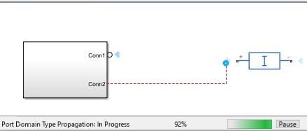
Port domain type propagation in progress, with Pause button on status bar.

Clicking Pause causes the following behavior:

Port domain type propagation is terminated, and resolved ports hold the correct port domain type and direction. Some percentage of ports might have an unresolved port domain type or direction. If you click Update Model from the Modeling tab or simulate the model at this time, propagation continues for the unresolved ports.
The editor is unlocked for use.
If you continue building your model, any subsequent complex propagation is terminated and is accompanied by a message indicating incomplete propagation.
A Resume button appears on the status bar.

Clicking Resume causes the following behavior:

Port domain types are computed for all ports affected since the last pause operation, including any complex propagation initiated after clicking Pause.
The Resume button is removed from the status bar.

Functionality being removed or changed

Hydraulic library will be removed

Still runs

Hydraulic library will be removed in a future release.

Compatibility Considerations

Use the Isothermal Liquid library and domain to model hydraulic systems where the working fluid temperature remains constant during simulation. Blocks in the Isothermal Liquid library provide increased accuracy, usability, and numerical performance. For more information, see Upgrading Hydraulic Models to Use Isothermal Liquid Blocks.

Simulation

Incremental Compilation: Reduce compilation time by recompiling only those parts of a model that have changed

Incremental compilation is an extension of the scalable compilation functionality. Scalable compilation lets you mark subsystems or blocks as reusable, and then reuses compilation artifacts for multiple repeated instances of a component in the same model. Incremental compilation reuses compilation artifacts of reusable components for subsequent compilations within the same MATLAB session, unless the component has been modified between simulation runs.

When you enable component reuse:

During the first compilation, the solver compiles one instance of each reusable component and then reuses these compilation artifacts for repeated instances in the model. This functionality is the same as in previous releases.
During subsequent compilations, the compilation time is further reduced because if a reusable component is unchanged, the solver does not recompile it. This optimization applies to all the reusable blocks and subsystems in the model, independent of whether there are multiple instances or just a single instance.

For more information, see Enable Component Reuse During Compilation.

The mechanism for marking subsystems or blocks as reusable has been consolidated and simplified. In previous releases, there were separate commands for marking subsystems and blocks as reusable and the command for subsystems applied only to referenced and linked subsystems. Now you can designate any subsystem or block as reusable:

simscape.reuse.setConfig(blockPath,'on')

where blockPath is the path to the block or subsystem from the root of the model.

To disable compilation reuse for a block or subsystem within a model, enter:

simscape.reuse.setConfig(blockPath,'off')

To query the reuse setting for a block or subsystem, enter:

setting = simscape.reuse.getConfig(blockPath)

Compatibility Considerations

The command-line interface for setting and getting the component reuse status has been consolidated and simplified. If you have scripts that use the old commands for setting and getting the block or subsystem status for scalable compilation, update them with the new command names and settings:

Instead of	Use
`simscape.scalable.setSubsystemConfig(blockPath,'auto')`	`simscape.reuse.setConfig(blockPath,'on')`
`simscape.scalable.setSubsystemConfig(blockPath,'off')`	`simscape.reuse.setConfig(blockPath,'off')`
`simscape.scalable.setBlockConfig(blockPath,'on')`	`simscape.reuse.setConfig(blockPath,'on')`
`simscape.scalable.setBlockConfig(blockPath,'off')`	`simscape.reuse.setConfig(blockPath,'off')`
`simscape.scalable.getSubsystemConfig(blockPath)`	`simscape.reuse.getConfig(blockPath)`
`simscape.scalable.getBlockConfig(blockPath)`	`simscape.reuse.getConfig(blockPath)`

Statistics Viewer Updates: Analyze simulation performance with the improved Statistics Viewer tool

The Statistics Viewer tool features an updated layout to enhance your analysis of model simulation statistics. To view model statistics, in the model window, on the Debug tab, click Simscape > Simscape Statistics. Using the tool, you can

View model statistics including information about the variables and zero-crossings
View statistics about the compilation process
Compare different models or model configurations

Now, when you select a block in the Statistics Viewer tool, you can highlight the block on the model canvas. The View Source button is available when you select a block that experiences a zero-crossing. The button takes you to the relevant equation in the source code.

To learn more, visit View Model Statistics.

Simscape to HDL Compatibility Enhancements: Use Trapezoidal Rule and real modes

You can now deploy HDL code from models with:

Solver type set to Trapezoidal Rule.
Operators floor, ceil, round, and mod without casting them as int32 or uint32.
Real-valued discrete variables. This update enables support for the Stepper Motor Driver (Simscape Electrical) block.

To learn more, visit Release Notes for HDL Coder (HDL Coder).

Improved Initialization Diagnostics: Avoid unexpected results when using OperatingPoint objects

Simscape now features improved handling for OperatingPoint object initialization. To learn more, visit Using Operating Point Data for Model Initialization.

Compatibility Considerations

You may generate different results from previous releases when initializing models with OperatingPoint objects.

New examples

Examples introduced in this version include: