R2025a

New Features, Bug Fixes, Compatibility Considerations

Simscape Language

 Declare composite domains

You can now declare a composite domain as a hierarchy of other, primitive or composite, domains. A primitive domain is a regular Foundation or custom domain that has nodes of a single type: electrical, gas, and so on. A composite domain is a textual equivalent of a bus port on a rigid Simscape Bus block. Composite domains have nodes that represent a bundle of connections, possibly of different types. For example, this composite domain combines two primitive domain types: mechanical translational and electrical.

domain MechElec
% Mechanical Translational and Electrical Domain
    nodes
        m = foundation.mechanical.translational.translational;
        e = foundation.electrical.electrical;
    end
end

To use a composite domain, design composite components with external ports that belong to that domain type. Connect these components to each other and to Simscape Bus or Connection Port blocks with corresponding rigid interfaces. For more information, see Composite Domains.

Use inverse hyperbolic functions in equations

You can now use these functions in the equations section and in simscape.Value objects:

• acosh — Inverse hyperbolic cosine.

• asinh — Inverse hyperbolic sine.

• atanh — Inverse hyperbolic tangent.

For a complete list of functions supported in the equations section, see Supported Functions.

Foundation Library

 Array Connection Block: Concatenate arrays of conserving connections into single array-of-nodes port

The new Array Connection block concatenates arrays of conserving connections into a single array-of-nodes (AON) port. Use the Array Connection blocks to connect individual elements, or subsets of elements, of AON ports of different sizes. You can also use this block to declutter a model diagram by bundling multiple connections of the same type and having two Array Connection blocks, facing each other, with their AON ports connected.

Probe Block: Probe across subsystem boundaries

The Probe block now has a dialog box, which you can use to connect the Probe block to another Simscape™ block, select which variables to probe, and customize the Probe port names and the output units for the variables.

In previous releases, the binding process involved double-clicking the Probe block and then clicking another block on the model canvas, and therefore you could connect the Probe block only to a block at the same level of the model hierarchy. Now, when you double-click a Probe block, its dialog box opens. Use the Connect button to attach (bind) the Probe block to another Simscape block, which can be located in a subsystem, or at any other level of the model hierarchy. Once you select the block, a list of its variables appears on the model canvas, as before. You can select the variables on the model canvas, or skip this step. Click Done connecting to complete the binding process. At this point, the Probe dialog box is populated with the list of variables from the attached block. If you selected any of the variables on the model canvas, they are selected in the dialog box as well. You can use the dialog box to continue selecting which variables to probe, customize the port names, and specify the output units, the same way as in the Property Inspector. The Property Inspector workflow, introduced in R2024b, and the process of selecting the variables directly on the model canvas work the same, as before.

During the binding process, when you navigate across the subsystem boundaries to a subsystem that is not open in a model tab, the Probe block dialog box can close automatically. In this case, you can end the binding process by clicking the X in the upper-right corner of the model canvas.

Cap (IL) Block: Terminate unused isothermal liquid ports

Use the new Cap (IL) block to terminate isothermal liquid ports on other blocks or to set the initial pressure at a node.

PS State-Space Block: Implement time-invariant linear state-space system

The new PS State-Space block, in the Physical Signals/Linear Operators library, implements a state-space representation of the linear time-invariant system.

Optional zero-crossings for Physical Signals library blocks

These blocks in the Physical Signals library now have an option to disable zero-crossing detection during simulation:

• PS Abs

• PS Dead Zone

• PS Max

• PS Min

• PS Ramp

• PS Saturation

• PS Switch

This change has no compatibility impact. By default, these blocks perform zero-crossing detection, like in previous releases. To improve simulation speed, you can disable zero-crossing detection for a block by clearing the Enable zero-crossing detection check box.

Optionally model dynamic compressibility and fluid inertia in Gas pipes

The Pipe (G) block has new options for modeling gas dynamics and fluid inertia:

• Enable dynamic compressibility — Select whether to account for the dynamic compressibility of gas. Dynamic compressibility gives the gas density a dependence on pressure, impacting the transient response of the system at small time scales. Disable dynamic compressibility if you want to reach steady state quickly during simulation or to simplify model initialization. By default, the block models dynamic compressibility, which is the same behavior as in previous releases.

• Enable fluid inertia — Select whether to account for the gas flow inertia. Flow inertia provides resistance to changes in mass flow rate. By default, the block does not model flow inertia, which is the same behavior as in previous releases. To enable the Enable fluid inertia check box, select the Enable dynamic compressibility check box.

Additionally, the block parameterization options have changed. Instead of specifying initial targets for block variables, you now specify initial parameter values and priorities in the Effects and Initial Conditions section.

To improve consistency, the names of the existing check boxes for modeling fluid compressibility and inertia in other Fluids domains have also changed to Enable dynamic compressibility and Enable fluid inertia.

Model ideal mutual inductor with no fast pole

The Mutual Inductor block has a new option that lets you model an ideal mutual inductor. If you select the Perfect coupling – no leakage checkbox, the block sets the coefficient of coupling to 1 and the leakage reluctances to 0. The block represents the ideal mutual inductor with no leakages and no fast pole, while also retaining the correct low-frequency behavior and blocking DC.

Spectrum Analyzer Block: Control plot type and use running averaging method

You can now individually control the type of plot for each line in the Spectrum Analyzer block. Select the line and set the Plot Type accordingly.

In R2025a, the Spectrum Analyzer block supports the running averaging method to compute the power spectrum estimate. To enable this mode, set the Averaging Method parameter to Running and the Spectral Averages parameter to a positive integer. For more information, see the Algorithms section in the Spectrum Analyzer block reference page.

 Use the Graph Data Extractor app to import data sheet graphs into MATLAB data files

The Graph Importer, introduced in R2024b, has been renamed the Graph Data Extractor. You can now access the Graph Data Extractor app from the Simscape section of the app library or by entering graphDataExtractor at the MATLAB^® command prompt. Use the app to import graphs from part data sheet PDFs, modify the point data, and then export the selected data as MATLAB data files. You can then use these data files to parameterize blocks.

To improve usability, the Graph Data Extractor app color scheme has been updated. The new colors improve accessibility.

 Compatibility Considerations

Previously, you opened the Graph Importer by entering graphImporter at the MATLAB command prompt. This command has been removed. Use the graphDataExtractor command instead.

 Name-Based Port Connections: Programmatically add connection lines between Simscape block ports

You can now programmatically add connection lines between physical modeling ports by using the port names. Supported block types include:

• Simscape blocks in the Foundation and Utilities libraries and in add-on product libraries

• Simscape Multibody™ blocks

• Subsystems that contain Simscape or Simscape Multibody blocks

For more information, see simscape.addConnection and simscape.connectionPortProperties.

 Compatibility Considerations

To provide consistent port naming for single-port blocks, the Solver Configuration block port name has been changed from A to port. This change can have a compatibility impact if you were using the Solver Configuration block inside a variant subsystem and referring directly to port A. To work around the issue, create another subsystem around the Solver Configuration block and refer from the variant subsystem to the external port name of this new subsystem. This solution makes the model more robust in case of other possible changes to the Solver Configuration block in future releases.

Connection Line Routing: Improved routing on addition or removal of block ports

Starting in R2025a, when you change a block parameter that exposes or hides a port, the existing connection lines do not change. If you add a port, the existing connection lines remain connected to their ports. If you remove a port, the corresponding connection line disconnects.

For example, in this model, port q of the Revolute Joint block connects to a Connection Port block, and port w connects to a Subsystem block. Port b does not connect to any block.

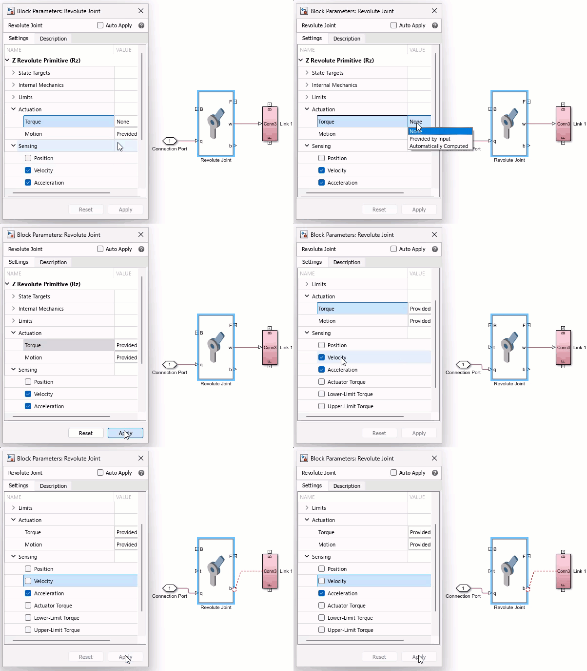
If you set the Torque parameter to Provided by Input, you expose the physical signal port t and the connection line between the Connection Port block and port q does not change. In previous releases, this connection line attached to port t.

If you clear the Velocity parameter check box, you remove port w and the connection line to the Subsystem block disconnects. In previous releases, this connection line attached to port b.

Block Data Sets: Create, manage, and store block parameter data

You can now parameterize Simscape blocks by using a block data set. The partrepo.simscape.BlockDataSet object stores part metadata parameter data that you can apply to a block. To generate a BlockDataSet object from a block, use the partrepo.simscape.dataSetFromBlock function.

Simscape uses JSON files to serialize the block data set. You can export block data sets to a JSON file or retrieve block data sets from an existing JSON file by using the partrepo.exportDataSetsToJSON function or the partrepo.importDataSetsFromJSON function, respectively.

To apply a block data set to a block, use the applyParams function.

To learn more, see Programmatically Manage Simscape Block Parameter Data.

Simscape Faults Enhancement: Reusable fault definitions

Reuse faults interactively by copying or cutting blocks that have faults assigned and pasting them. Use this feature to add faults to libraries for reuse. To learn more, see Copying Faults.

 Functionality being removed or changed

Models that contain Hydraulic library blocks display warnings

Warns

When you run a model that contains Hydraulic library blocks, the model displays a warning. The Hydraulic library will be removed in a future release. To suppress this warning, select Suppress hydraulics deprecation warning in the Hydraulic Fluid block.

 Compatibility Considerations

Use the hydraulicToIsothermalLiquid function to upgrade your hydraulic models to use isothermal liquid blocks. Blocks in the Isothermal Liquid library provide increased accuracy, usability, and numerical performance.

Use the new subsystemflag argument to minimize the number of blocks placed into subsystems when you run the hydraulicToIsothermalLiquid function. Previously, the hydraulicToIsothermalLiquid function placed many hydraulic blocks into subsystems to reduce the impact of signal rerouting. Now, you can use the subsystemflag argument to control the subsystems the block makes. By default, subsystemflag is "omitsubsystems", and the function only uses subsystems if the function replaces a single Hydraulic block with multiple Simscape blocks. Even when subsystemflag is "omitsubsystems", in many models line rerouting is minimal. If you specify subsystemflag as "addsubsystems", the function places blocks that impact line routing into subsystems to fully preserve the Hydraulic model line routing.

Default parameter values of the Thermal Liquid Settings (TL) block have been adjusted

Behavior change

The default parameter values of the Thermal Liquid Settings (TL) block have been adjusted to match the corresponding values in the domain file:

• Maximum valid temperature changed from 363.16 K to 373.16 K.

• Minimum valid pressure changed from 0.05 MPa to 0.01 MPa.

This change has no compatibility impact. If your model contains a Thermal Liquid Settings (TL) block from a previous release, its parameter values do not change.

Simulation

 DAE Solver: Run-time parameter performance improvements

Simulation time may improve when you simulate a model with run-time parameters using a DAE solver. The solver uses improved logic to handle run-time parameters when, in the Solver Configuration block, you select Use local solver.

Scalable Compilation: Skip the baseline compilation

For scalable compilation, the Advisory tool lets you analyze your model for unsupported patterns, provides compilation statistics, and makes recommendations on whether to enable scalable compilation. To do this, the tool compiles the model twice: first, without scalable compilation, to calculate the baseline, and then again with applying scalable compilation.

However, after you have decided to enable scalable compilation, you can still use the Advisory tool to try different ways of restructuring your model into repeated components, to optimize the configuration. In this case, you do not need to calculate a baseline, because you are interested only in the scalable compilation statistics for the current configuration. To save time, you can skip the baseline compilation by using this syntax:

sscScalableAdvisor(modelname,subsyspaths,CompareBaseline=false); 

where:

• modelname is the name of the model to analyze, specified as a character vector, string, or a handle to the model. This argument is required.

• subsyspaths is an optional argument that identifies the repeating subsystems in the model.

For more information, see sscScalableAdvisor.

Scalable Compilation: Enhanced support of nonlinear index reduction

Scalable compilation now supports the derivative replacement method of nonlinear index reduction. Nonlinear index reduction is a global transformation used for solving high-index nonlinear equations. In R2024b, only the projection method was supported. For more information, see the Index reduction method parameter of the Solver Configuration block.

 Compilation Speed Enhancement: Declaration function caching

Many Simscape blocks, such as heat exchangers or bipolar transistors, use declaration functions to compute derived parameter values and initialize variables. Previously, these computations were performed every time the model was compiled. Now, the computation results of declaration functions are included in the cached model compilation artifacts. This enhancement speeds up model compilation because the parameter and variable values do not need to be recomputed, unless the underlying block parameters have changed.

 Compatibility Considerations

If your custom block uses a declaration function for random number generation, caching can lead to unexpected simulation results because the values are reused for subsequent simulation runs and therefore are no longer random. If your model relies on a declaration function generating random parameter or variable values at every simulation run, you can use the new Cache compilation artifacts model configuration parameter to turn off caching.

This restriction applies only if you use functions like rand, randi, or randn inside a MATLAB declaration function. If you call rand, randi, or randn directly from Simscape code, for example, use it in a Simscape function or directly in a parameter declaration, caching does not apply.

 Improved handling when simulating with local solvers

Local solver enhancements improve simulation time for some models when, in the Solver Configuration block, you select Use local solver and clear Resolve indeterminate equations during runtime. Generated code now has improved performance with a smaller footprint.

 Compatibility Considerations

Simulation results may differ slightly from previous releases.

Refine output to avoid spikes at zero crossings

Use the new model configuration parameter on the Solver pane, Continuous state refinement method, to refine output and avoid spikes at zero crossings:

• Solver interpolation (default) — Use solver interpolation between major steps for zero-crossing detection and state refinement. This behavior is the same as in previous releases.

• Solver stepping — Use the solver discretization method, effectively taking shorter steps between the major steps and applying the solver discretization formula at refined points. This option has higher computational cost but may produce a solution that better satisfies the equations and avoids spikes at zero crossings.

To enable this parameter, set the Solver parameter to daessc (DAE solver for Simscape).

Operating Point Enhancements: Display operating point data in table format

You can now use the simscape.op.targetTable function to generate a MATLAB table display of a Simscape operating point data for visual inspection or programmatic access. To generate an operating point table, use the syntax:

opTable = simscape.op.targetTable(op);

The simscape.op.targetTable function takes a Simscape operating point, op, and returns the MATLAB table, opTable.

Simscape-to-HDL: Generate fixed-point bitstreams and improved implementation models

When you use Simscape-to-HDL code generation, you can now:

• Generate FPGA bitstreams from Simscape models with tunable run-time parameter values when, in the Solver Configuration block, you select Use local solver and set Solver type to Trapezoidal.

• Generate improved HDL-optimized models when you use the sschdl.generateOptimizedModel function.

To learn more about R2025a Simscape-to-HDL features, see Release Notes for HDL Coder (HDL Coder).

New examples

Examples introduced in this version include:

• A Comparison of the Mutual Inductor and Ideal Transformer Library Blocks

• Cooling Plate With Channels

• Heat Sink Using PS State-Space Block

• Angle-Based Mechanical Rotational Systems

 Functionality being removed or changed

Improved equation scaling

Behavior change

Enhancements and optimizations for run-time scaling of equations in this release result in better simulation robustness. Certain poorly scaled models where the solver previously failed to find a solution now simulate successfully.

 Compatibility Considerations

Because of equation scaling optimizations, there may be slight differences in simulation results compared to R2024b.