R2023a

New Features, Bug Fixes, Compatibility Considerations

Simulink Editor

Open Simulink models with invalid names

You can now open a model even when the file does not have a valid name, for example, mymodel (1).slx. Simulink^® opens the model and assigns a valid name. To rename or save changes to the newly named model, click Save. For more information, see Choose Valid Model File Names.

Enhancements to suppression manager user interface

You can now add inline comments to suppressed warnings. You can also filter diagnostic messages, suppression location, and comments using a global filter. The look and feel of the suppression manager is also enhanced.

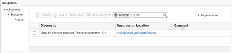
For more information, see Suppress Diagnostics

 Functionality being removed or changed

Removed warning and corrected keyboard shortcut actions for comment-out and comment-through operations

Behavior change

The comment-out and comment-through workflows have been updated:

• Commenting out or commenting through a group of blocks does not issue a warning for the blocks that do not support these operations.

  • If you select a combination of blocks that support and unsupport commenting out or commenting through operations, Simulink comments only the supported blocks. The unsupported blocks are silently skipped.

    

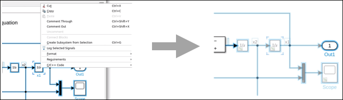
  • If all the blocks that you select do not support commenting, the Comment Out and Comment Through options are disabled.

  • If the blocks that you select are already commented out, the Comment Out option is disabled.

  • If the blocks that you select are already commented through, the Comment Through option is disabled.

  In previous releases, these actions issued a warning for unsupported blocks and continued to comment the supported blocks.

• The keyboard shortcuts Ctrl+Shift+X and Ctrl+Shift+Y failed to uncomment a group of commented-out and commented-through blocks if the selection included one or more unsupported blocks. These shortcuts now work properly.

For models created before R2010b, Simulink no longer renames blocks that only differ in white space type

Behavior change

In R2023a, Simulink no longer renames blocks that only differ by the type of the white space. The same subsystem cannot contain two different blocks that only differ in the white space type, for example and . This was only possible for models created before R2010b.

For models created in R2010a and earlier, Simulink warns when attempting to load the blocks that only differ in white space type. Rename the block in a previous release and save the model.

Simulation Analysis and Performance

Step simulation block by block using new options in the Simulink Editor

In previous releases, when you simulated a model that contained signal breakpoints, the simulation paused at the end of the major time step in which the condition for the signal breakpoint was met. Starting in R2023a, by default, the simulation pauses within the time step as soon as the condition is met. Once the simulation pauses within the time step, new stepping buttons on the Debug tab of the Simulink Toolstrip become active and allow you to step through the simulation execution one block at a time. As you step through a simulation block by block, you can use port value labels to view signal values in the block diagram.

In addition to the enhanced capabilities for signal breakpoints, you can now add zero-crossing and Inf or Nan value model breakpoints using the Simulink Toolstrip.

For more information about the new stepping and breakpoint options, see Breakpoints List.

These additions replace the standalone Simulink Debugger. The Simulink debugging programmatic interface remains unchanged for programmatic simulation debugging.

Add breakpoints and access help from the Breakpoints List

The Breakpoints List has two new buttons:

• To add a signal breakpoint from the Breakpoints List, select a signal then click Add Breakpoint .

• To access documentation, click Help .

In addition to the new buttons, you can use the new Pause within time step option to control whether the simulation pauses within a time step as soon as the condition for a breakpoint is met or pauses at the end of that time step. For more information, see Breakpoints List.

Performance improvement for simulations with back stepping enabled

Enabling stepping back in simulation has a smaller effect on simulation performance. To support stepping back in simulation, the software captures simulation snapshots, which adds overhead and can slow simulation. The performance improvement for simulations with stepping back enabled varies between models, with smaller improvements for models that use certain blocks and features, including:

• Referenced models configured to simulate in accelerator mode

• Simscape™ blocks

• S-functions that implement custom methods for saving and restoring the S-function operating point

You can assess the performance improvement for a model by running equivalent simulations of the model in R2022b and R2023a with back stepping enabled and checking the execution time in the simulation metadata. For example, to assess the performance improvement for the model slexAircraftExample, follow these steps using R2022b and then R2023a:

1. Open the model.

   openExample(...
       "simulink_aerospace/AircraftLongitudinalFlightControlExample",...
       supportingFile="slexAircraftExample")

2. To capture timing information in the simulation metadata, including the time spent in the execution phase of the simulation, check that the Single simulation output parameter is enabled.

   In the Simulink Toolstrip, on the Modeling tab, click Model Settings. On the Data Import/Export pane, select Single simulation output.

3. Enable stepping back.

   On the Simulation tab, click Step Back. In the Simulation Stepping Options dialog box, select Enable stepping back.

4. In the Simulation Stepping Options dialog box, check that the Maximum number of saved back steps and Interval between stored back steps parameters both use the default value of 10. Then, click OK.

5. Use the same start and stop times for the simulation in R2022b and R2023a. For this simulation, use a stop time of 1000 seconds.

   On the Simulation tab, in the Stop time field, enter 1000.

6. To run the simulation, on the Simulation tab, click Run.

7. Check the execution time in the simulation metadata captured in the simulation output.

   execTime = out.SimulationMetadata.TimingInfo.ExecutionElapsedWallTime;

The table summarizes performance improvements for two example models by comparing the execution time between simulations run in R2022b and R2023a. The model asbhl20 shows a smaller performance improvement because the model uses features that involve custom operating point implementations, including a referenced model that simulates in accelerator mode. The simulations were timed on a Windows^® 10, AMD^® EPYC 74F3 @ 3.19 GHz test system.

Model Name	Simulation Duration	Approximate Execution Time in R2022b	Approximate Execution Time in R2023a	Approximate Execution Time Improvement
slexAircraftExample For more information about the model, see Aircraft Longitudinal Flight Control.	0 to 1000 seconds	2.3 s	1.0 s	56%
asbhl20 For more information about the model, see HL-20 Project with Optional FlightGear Interface (Aerospace Blockset).	0 to 61 seconds	760 s	650 s	14%

For more information about how stepping back and the simulation stepping options affect simulation performance, see How Stepping Through Simulation Works.

Execution Order pane enhancements

Starting in R2023a, the Execution Order pane:

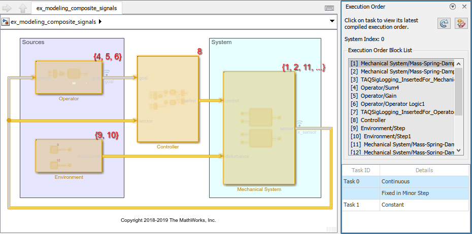
• Lists the task-based execution order of blocks, including hidden blocks. Previously, the execution order was displayed only on visible blocks. The block list provides complete execution order information for the selected task.

• Uses the latest compiled execution order for a model. Previously, opening the execution order pane compiled the model regardless of whether the model was already compiled. Now, to recompile a modified model, click Recompile model to update execution order information .

For more information, see Control and Display Execution Order.

Usability improvements in the Simulation Data Inspector

The Simulation Data Inspector has several improvements to help you control the visualization of signals for better data analysis.

• When you add new signals to a plot, you can now choose to preserve axes scaling or automatically scale axes limits to view the newly added data. Previously, axes limits were always automatically scaled when you added new signals to a subplot.

• Access subplot-specific operations, such as performing a fit-to-view in y for an individual subplot, from the context and subplot menus.

• Live streaming improvements allow you to change the time span and time axis limits in an intuitive way. Previously, changing the time axis limits during live streaming also changed the time span. Now, the time span remains fixed when you change the minimum or maximum time axis limit. When you change the time span during live streaming, the minimum time axis limit remains the same and the maximum time axis limit adjusts such that t-Axis max = t-Axis min + Time span.

• The Import dialog box now has an option to select all or none of the check boxes when importing data from the workspace or a file.

Improved signal selection for XY plots

With the improved XY Data dialog box, you can easily add and manage signals in XY plots. Previously, you had to use the Shift or Ctrl key to select more than one signal from the signal table then drag the signals onto the XY plot.

Now you can select multiple check boxes in the signal table to add signals to the XY Data dialog box. Then, use the x-Axis and y-Axis drop-down menus to manage how signals are paired for easy plotting.

You can also now perform a fit-to-view in x or y when viewing data in an XY plot.

Log nonvirtual buses that contain variable-size signals

In normal and accelerator mode simulation, you can now log:

• Nonvirtual buses that contain variable-size signals directly or in nested buses

• Buses with nested nonvirtual buses that contain variable-size signals

In normal mode simulation only, you can now log:

• Arrays of buses with nonvirtual buses that contain variable-size signals

Set signal comparison constraints programmatically

Use name-value arguments to set comparison constraints like the sensitivity to data type, time vector, or start and stop times when comparing two signals programmatically. For more information, see Simulink.sdi.compareSignals.

Load MLDATX files and export data using the Playback block

There are two enhancements to the Playback block in R2023a:

• In R2022b, you could add data to the Playback block from the workspace, a file, and the Simulation Data Inspector, but you could not aggregate and export that data outside the Simulink environment. Now, you can take data that has been added to the Playback block from different sources (linked to from the source or saved in the model) and export that data to the workspace or a file.

• The Playback block now supports loading data from a Simulation Data Inspector session file. Adding data from a native MLDATX file format speeds up loading time and allows you to selectively load individual signals from large data sets.

Access diary information for simulations running with parsim

Starting in R2023a, you can access diary information about simulations that run on parallel workers. When running simulations with parsim, you can access the information about warnings, status updates, or user-printed messages. To access this information, use the Diary field in the ExecutionInfo struct of the SimulationMetada property of each Simulink.SimulationOutput object.

Pause complex port domain type propagation for Simscape blocks

For Simscape blocks, port domain type propagation is the process that computes port domain types of all linked connection ports. In complex models where propagation can take longer to complete, the Simulink editor is locked for editing. Starting in R2023a, you can suspend propagation and resume editing the model by clicking the Pause button on the status bar.

For more information, see Port Domain Type Propagation: Speed up editing complex models (Simscape).

 Functionality being removed or changed

get function for Simulink.SimulationOutput object issues error if specified property does not exist on object

Behavior change

Prior to R2020a, the get function returned empty ([]) if the specified Simulink.SimulationOutput object did not have the specified property. Since R2020a, the get function has issued a warning while still returning empty in this situation. Starting in R2023a, the get function issues an error and does not return an output argument.

To query whether a Simulink.SimulationOutput object has a given property, use the find function. The find function returns empty ([]) and does not issue a diagnostic when the object does not have the specified property.

Component-Based Modeling

Use local solver for model reference at any location in model hierarchy

Starting in R2022a, you could configure a Model block in the top model of a model hierarchy to use a local solver to compute results for the model reference. In R2023a, you can configure a Model block anywhere in a model hierarchy to use a local solver, including Model blocks inside model references that use local solvers.

Expression mode support and dialog box updates in Variant Assembly Subsystem block

You can use Boolean conditional expressions to switch between variant choices of Variant Assembly Subsystem blocks. Using conditional expressions enable you to change the active choice during different stages of simulation and code generation without modifying the block. You can generate code that contains active and inactive choices with meaningful names.

In the Variant Assembly Subsystem block dialog box, you specify a variant control variable and an enumeration class with model or subsystem filenames as its members. On successfully validating these parameter values, the block adds the enumerated members as its variant choices and generates conditional expressions for each of its choices. To add more variant choices, add members to the enumerated class. To remove variant choices, delete corresponding members from the enumeration class. For more information, see Add or Remove Variant Choices of Variant Assembly Subsystem Blocks Using External Files.

Previously, you could use only labels to switch between variant choices.

To support the expression mode, the block dialog box has been reorganized:

• The Main and Reference tabs are merged. All the parameters in these tabs are placed in the same space. The Variant choices table in the Reference tab is removed.

• A Variant Assembly section is added for variant assembly related actions. The newly introduced parameters Variant control variable and Variant choices enumeration parameters are available in this section. These parameters support expression mode workflows.

• The Validate button is no longer available to evaluate the variant choices specifier that you specify. Instead, click the Refresh button to evaluate the specifier. In expression mode, the values that you specify for Variant control variable and Variant choices enumeration are evaluated on clicking the Refresh button.

Identify potential inconsistencies in variant choices controlled from mask or model workspace

You can identify potential inconsistencies in the choices of variant blocks that are controlled from mask parameters or from mask or model workspace variables early in the development process during the update diagram. Early detection saves you valuable time and improves product quality. To enable early detection, set the Variant activation time parameter of the variant block to update diagram analyze all choices. For more information, see Approaches to Control Active Variant Choice of a Variant Block Using Mask or Model Workspace.

Previously, you could analyze such variant choices only in the later stages of the development process.

Conditionalize insertion options and create subsystem choices with adaptive interfaces inside Variant Subsystems

When you drag a selection box around an empty area inside a Variant Subsystem block, the action bar shows choice insertion options that are based on the type of subsystem choices in the block. From these options, select Variant Subsystem Choice to add a new subsystem choice. The subsystem choice that you create adapts its interface from the Variant Subsystem block. The choice has the same number and types of input and output ports as the Variant Subsystem block. For more information, see the "Include Subsystem Block as Variant Choice" section in Implement Variations in Separate Hierarchy Using Variant Subsystems.

Previously, the options in the action bar were not conditionalized. Also, the newly created subsystem choice had only one input and one output port.

Support for continuous states with startup variant blocks

You can now simulate and generate code for startup variant blocks that are connected to continuous state blocks. Previously, you could use startup variant blocks only with discrete blocks. For information on the capabilities of startup, see startup.

Group variant parameter values in a single structure array in generated code

Use variant parameter banks to group variant parameters that share the same variant conditions into a structure in the generated code. A simple pointer switching mechanism enables you to switch the set of active parameter values in the code based on variant conditions. You can set code generation properties for the variant parameter bank which allows you to customize code placement and specify the memory section to place the parameter values in the compiled code. Variant parameter banks are supported only for variant parameters with startup variant activation time.

The code that you generate using Embedded Coder^® contains all choice values grouped into a structure array based on the variant conditions. The code uses a pointer variable to access values from the structure array; this pointer is initialized based on variant conditions in the model_initialize function. Parameter bank switching using a pointer variable avoids copying the choice values into the main program memory and improves the efficiency and readability of the generated code.

Previously, for variant parameters with startup activation time, the values of the parameters were inlined in the model_initialize function in the generated code, which involved reading and copying all parameter values into the program memory. This behavior is still applicable when you generate code using Simulink Coder™.

For more information, see Simulink.VariantBank and Simulink.VariantBankCoderInfo.

Enhancements to the Variant Manager for Simulink support package

• Manage variant parameters from Variant Manager

  The model hierarchy table shows variant parameters available in the workspace used by the model in a new tab view named Variant Parameters. You can edit the Condition and Value properties from the model hierarchy table or use the context menu to open the Simulink.VariantVariable dialog box to edit the properties.

• Improved user interactions in the Control Variables table

  • Autocomplete control variable names on typing in the Name column.

  • Filter table rows based on a search string.

  • Show or hide the VAT and Source columns in the table.

• Improved name and tooltip for Stateflow^® variant transitions

  The Stateflow view indicates the source and destination states of a variant transition in the Name column and shows additional information in the tooltip.

• Support for startup variant activation time in Variant Reducer

  When you reduce a model that contains a variant block with startup activation time, Variant Reducer retains the block and any blocks connected to it in the reduced model. Previously, reduction of such models resulted in an error.

Programmatically refresh variants, linked blocks, and Model blocks

Starting in R2023a, you can use the Simulink.BlockDiagram.refreshBlocks function to programmatically refresh all variants, linked blocks, and Model blocks in a loaded model.

This function provides a programmatic alternative to the Refresh Blocks button in the Simulink Toolstrip. This button is on the Modeling tab under the Update Model button arrow.

The Model blocks update only when the Model block version mismatch and Port and parameter mismatch configuration parameters are set to none or warning. The Model blocks do not update when either configuration parameter is set to error.

To refresh blocks in referenced models, call this function for each referenced model.

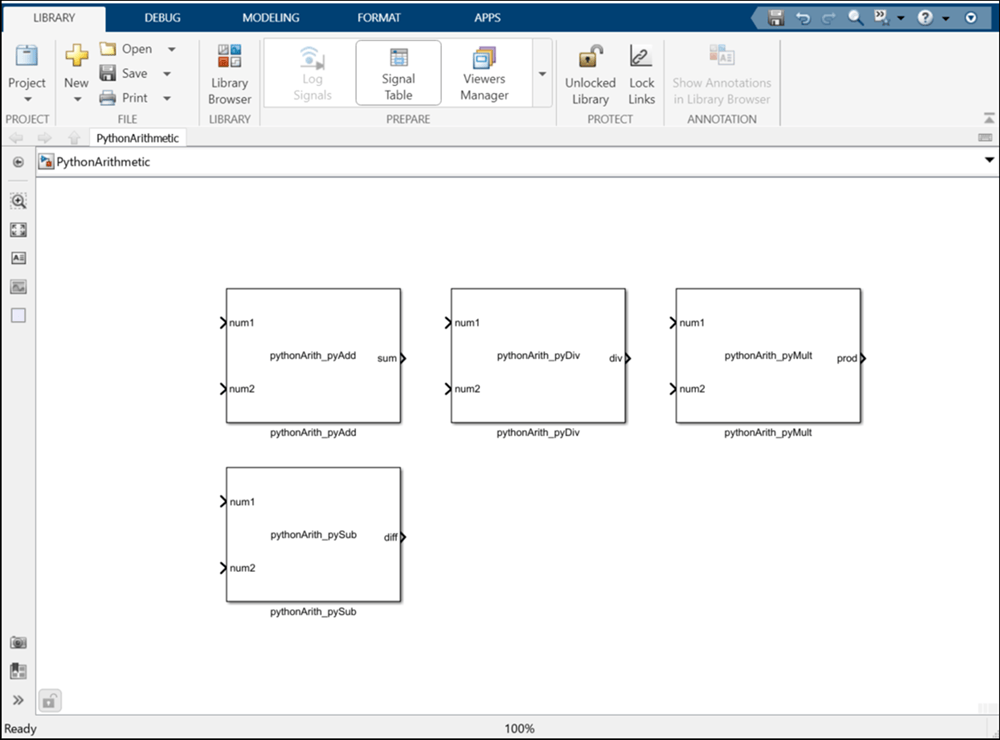
Integrate Python functions with Simulink using Python Importer

Starting in R2023a, you can integrate Python^® functions with Simulink using the Python Importer within Blockset Designer. Use this feature to import python functions and packages to Simulink and generate a custom block for each function.

Specify Python files containing one or more function definitions in Files to import or Python packages containing one or more Python files in Packages to import. You can also specify a directory containing files to include in the package published by Blockset Designer in Python Folder.

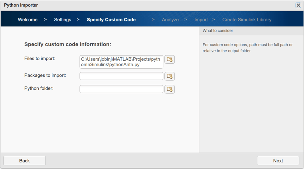
The Python Importer identifies all the functions specified in the Python files. You can select the functions for which the importer creates a custom block inside a Simulink library.

You can use the blocks from the library in your model or publish the blocks as a blockset using the Blockset Designer.

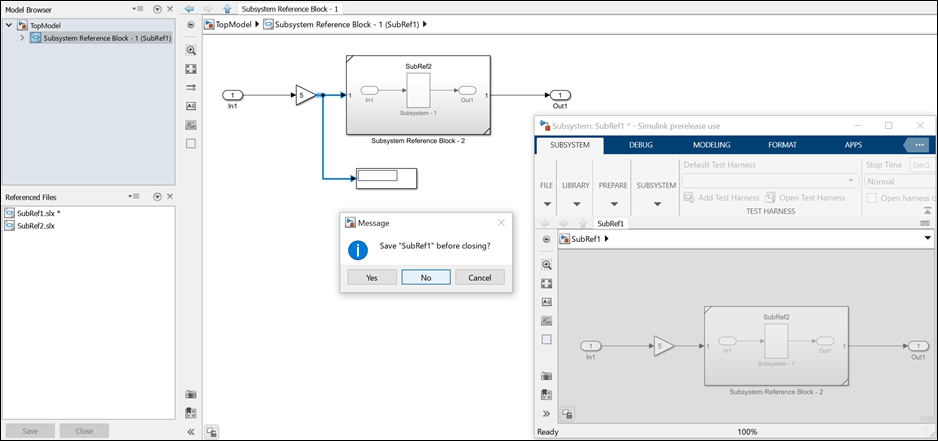
Discard changes in individual subsystem files without reversing all modifications in a model

The changes that you make to a particular subsystem file from its instance can be locally discarded. Previously, you could reverse your actions to get back to a desired state, but this process discarded all changes made in any of the subsystem files within the model hierarchy.

For example, to discard the changes in subsystem file SubRef1 made while editing its instance Topmodel/Subsystem Reference Block-1, close SubRef1. You will get a dialog box asking whether to save the subsystem file before closing. Click No. This action reverts changes in all the instances of the subsystem file.

Initial state parameter ignored for referenced models in normal mode

Starting in R2023a, for referenced models that simulate in normal mode, simulation ignores the Initial state configuration parameter.

Support for web browser display widget in mask editor

Starting in R2023a, the mask editor supports the web browser display widget. Enter the address in the URL property. The website opens in a preview of the dialog box.

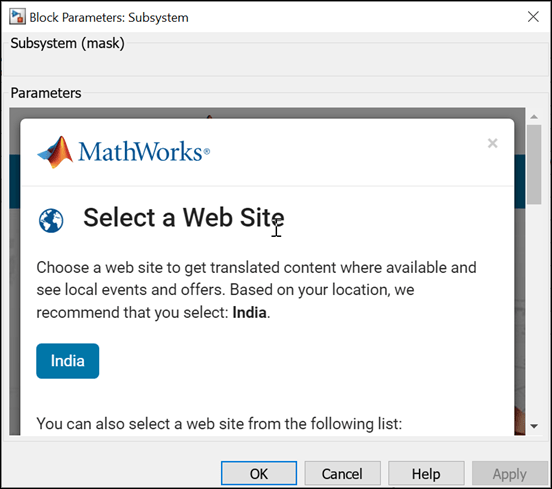
For more information, see Controls

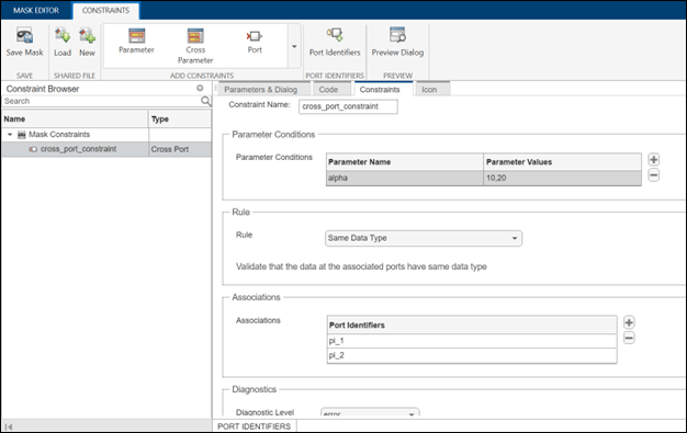
Create cross-port constraints to validate signals among ports of the same masked block

Starting in 2023a, you can create cross-port constraints among input and output ports of the same masked block. The predefined rules available are Same Data Type and Same Dimensions. For example, you can constrain the input and output port signals to be of same data type. You can also set parameter conditions with mask parameters while defining cross-port constraints. The cross-port constraints are validated when you compile the model.

To create cross-port constraints, specify the name of the constraint, then set the rules and parameter conditions appropriately.

Organize mask callbacks and initialization code in a MATLAB file

Starting in R2023a, you can write mask initialization, parameter, and dialog control callbacks in a separate MATLAB class file instead of storing it with the mask object. The advantages of using a MATLAB file are:

• Organization of all mask callbacks in a single file.

• Enhanced debugging experience. You can use all code debugging capabilities provided by the MATLAB editor, such as breakpoints, to debug your initialization and mask callback code.

• Improvement of the memory footprint of the masks, as callbacks are no longer in memory but rather are in a MATLAB file on the disk.

• Ability to edit the mask callback code using either the mask editor or the MATLAB editor.

• Option to package the MATLAB class file along with the model.

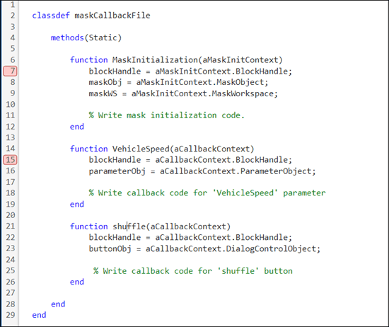
For more information, see Organize Mask Initialization and Callbacks in a MATLAB File

Authenticate usage and code reusability of your subsystem files in top model

Subsystem components are adaptable to environments. However, you can get undesired results if you use a component out of context. In R2023a, you can mark the test environments of a subsystem file that produce the intended results as unit tests.

Use the Unit Test features available in the Simulink toolstrip to:

• Specify valid testing environments.

• Capture signatures to diagnose and resolve invalid use of components.

• Generate code for subsystem components to re-use in the top model.

For more information, see Validate Subsystem Reference Use and Build Model Using Component Codes.

Create self-modifiable referenced subsystems using mask initialization code

You can now make instance-specific changes in the contents of a masked subsystem file using the initialization callback of the system mask. To make changes, set the subsystem file as self-modifiable. In a self-modifiable subsystem file, you can:

• Modify the blocks inside a masked subsystem reference instance.

• Allow the masked subsystems inside a masked subsystem reference instance to self-modify.

For more information, see Create Self-Modifiable Subsystem Reference Using System Mask.

Simulink unit updates

Simulink units now support these prefixes as announced at the 27th meeting of the General Conference on Weights and Measures (CGPM).

Prefix	Factor	Symbol
quecto	10-30	q
ronto	10-27	r
quetta	1030	Q
ronna	1027	R

 Functionality being removed or changed

Variant blocks issue warning when blocks do not inherit variant activation times from their Simulink.VariantControl variables

Warns

Starting in R2023a, variant blocks issue a warning if the blocks do not inherit the activation times from their variant control variables of type Simulink.VariantControl, if any. All the Simulink.VariantControl variables of a variant block must have the same activation time. In previous releases, the blocks did not issue the warning.

If this change impacts your model, set the Variant activation time of the variant blocks to inherit from Simulink.VariantControl.

For more information, see inherit from Simulink.VariantControl.

Define shared constraints in XML file

Warns

Starting in R2023a, you can define the shared constraints in XML files. The advantages of defining in an XML file are that you can edit the data and compare the file with a previous version. If you have shared constraints authored in a MAT-file, you can convert it to an XML file using the method Simulink.Mask.Constraints.convertMatToXML(<matFilleName>, <xmlFileName>). matFileName is the name of the MAT file to be converted and xmlFileName is the name of the XML file to be created. Simulink no longer allows you to define the shared constraints in MAT files. However, the existing constraints continue to work until you open the mask editor.

For more information, see Share Parameter Constraints Across Multiple Block Masks

lcc-win64 compiler will be removed

Still runs

The lcc-win64 compiler will be removed in a future release. For information about supported compilers, see Supported and Compatible Compilers - Windows.

Project and File Management

Dependency Analyzer: Perform a block-level dependency analysis

You can now perform a block-level dependency analysis for your project or model hierarchies. For an example showing how to identify the impact of changing a single block on the other files in your design, see Perform Block-Level Impact Analysis Using Dependency Analyzer.

Dependency Analyzer: Analyze files and folders with or without a project

Starting in R2023a, you can access Dependency Analyzer from the MATLAB^® Apps gallery. You can now perform a dependency analysis on files and folders that do not belong to a project. For more information, see Dependency Analyzer.

Project Preferences: Recreate empty project folders in Git repositories

Git™ does not track empty folders and ignores them when you commit. MATLAB now enables you to recreate an empty folder structure in a project under Git source control. Doing so is useful for small projects intended for training or as procedure templates.

For large projects, to avoid performance issues on startup, clear Recreate empty project folders in a project under Git. For more information, see Set MATLAB Projects Preferences.

Project API: Determine if file is under project root folder

You can now programmatically determine whether a file or a folder is under a project root folder by using the matlab.project.isUnderProjectRoot function.

Project API: Export subset of project files to archive

You can now programmatically export a subset of project files to an archive by specifying a user-defined export profile in the export function.

Project Sharing: Include only specific files in project archive using export profile

You can now use an export profile to include only files with particular labels in a project archive. This option is useful if the files you need to share are only a small subset of a large project. For more information, see Archive Projects.

Model Comparison: Save printable reports without screenshots

You can now save comparison reports without screenshots. Before you save the comparison results as a printable report, in the Command Window, enter:

s = settings().comparisons.slx.DisplayReportScreenshots;
s.TemporaryValue = false;

For more information, see Save Printable Report.

Text Comparison: Automate comparison report generation for continuous integration (CI) workflows

Starting in R2023a, you can programmatically publish comparison reports for plain text files, MATLAB scripts, and text-based source code files. Automate report generation for continuous integration (CI) workflows using the visdiff function:

comparison = visdiff(textfile1,textfile2);
file = publish(comparison);
web(file)

Text Comparison: Save comparison results as PDF or DOCX reports

You can now use the Comparison Tool to publish text comparison results as PDF or DOCX reports. For more information, see Compare Text Files.

Source Control in MATLAB Online: Detect and extract conflict markers from text and binary files

In MATLAB Online™, you can now detect conflict markers added by Git in text and binary files. Extract conflict markers to repair corrupted files.

Source Control in MATLAB Online: Save uncommitted changes by creating a Git stash

In MATLAB Online, you can now save uncommitted changes by creating a Git stash.

Source Control in MATLAB Online: Manage Git remote repositories locally using Branch Manager

In MATLAB Online, you can now manage multiple remote repositories from a local Git repository. Use Branch Manager to perform these tasks:

• Add, edit, and delete remote repositories.

• Fetch from all remotes or individual remotes.

• Prune remote branches from all or individual remotes.

• Open selected remotes in a web browser.

• Create new local branches that track remote branches.

• Delete remote branches.

Project Comparison in MATLAB Online: Compare project definition files

Starting in R2023a, when you compare folders in MATLAB Online, MATLAB detects whether they are project root folders. MATLAB looks for and compares the project definition files stored in the resources or .SimulinkProject folder. Project definition files contain information about the project path, project settings, shortcuts, labels, and referenced projects. For more information, see Compare MATLAB Projects in MATLAB Online.

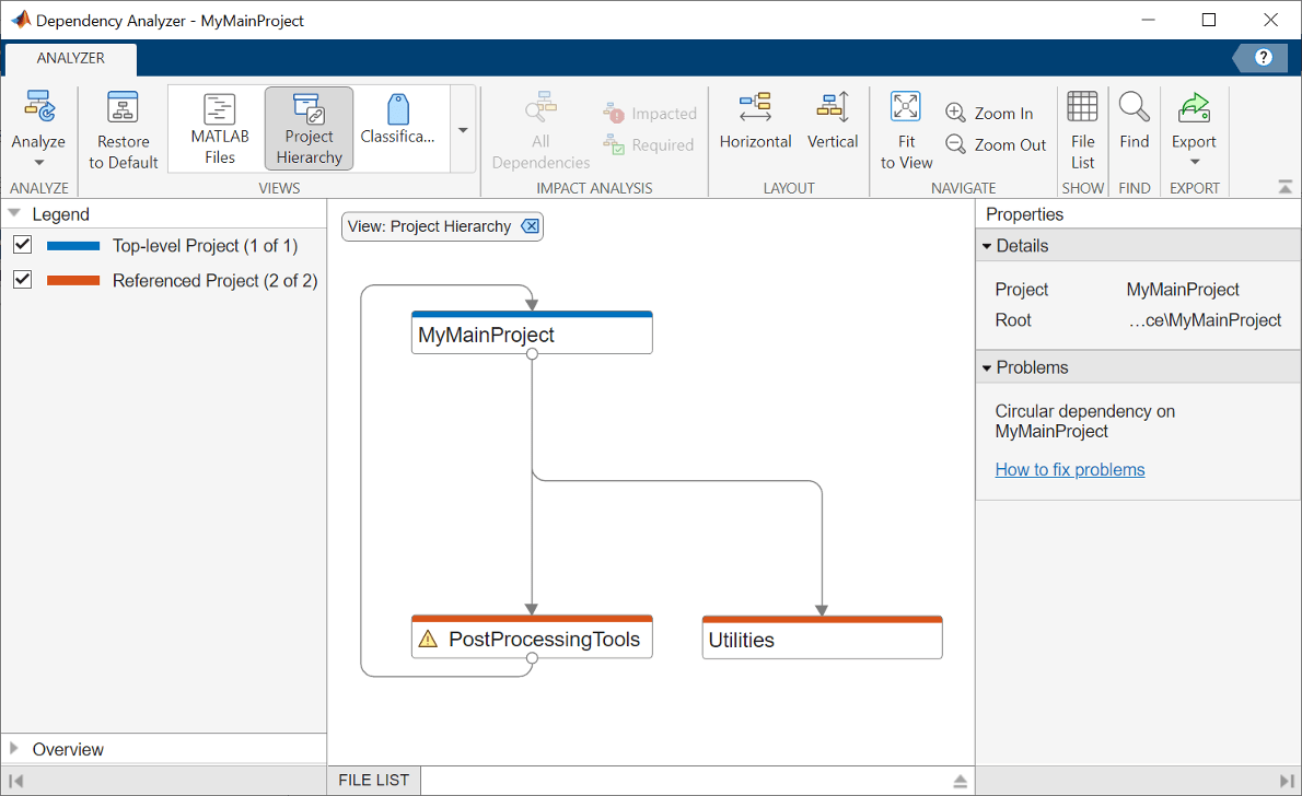
Dependency Analyzer in MATLAB Online: Investigate circular dependencies using the Project Hierarchy view

You can now investigate how projects in your hierarchy relate to each other and identify projects that introduce circular dependencies using the Project Hierarchy view in MATLAB Online. For more information, see Explore the Dependency Graph, Views, and Filters.

 Functionality being removed or changed

XML comparison type will be removed in a future release

Still runs

XML comparison type will be removed in a future release. Overriding the default comparison type by specifying "xml" will not be possible in a future release. In R2023a, scripts that use visdiff(filename1,filename2,"xml") continue to work. See visdiff.

Data Management

Signal Editor tool updates

The Signal Editor tool has these updates:

• Import and Export commands now appear directly on the toolstrip in the File section. In previous releases, these commands were contained in the Save and Open menus, respectively.

• Snap to incremental values in the X and Y grids.

Root Inport Mapper updates

The look and feel of Root Inport Mapper has changed. Continue to use it as in previous releases. Changes include:

• The link from MAT-file shortcut Ctrl+Shift+M has changed to Ctrl+Shift+L.

• Root Inport Mapper icons have changed slightly.

  Action	Old Icon	New Icon
  Open
  Save
  Save As
  From Spreadsheet
  From MAT-file/Edit MAT-file
  From Workspace
  Signals
  New MAT-file
  Options/defaults
  Map All
  Map Selected
  Map Unconnected
  Map Failed
  Map Warned
  Apply to Model
  Generate Script

Simulink.ValueType object enhancements

Starting in R2023a, Simulink.ValueType objects:

• Support Simulink.Bus objects as data types. When the value type specifies a bus object data type and a nonscalar dimension, the value type specifies an array of buses.

• Are supported as data types of Simulink.Signal and Simulink.Parameter objects.

Package Simulink data dictionary with referenced subsystems for better reusability and scoping

You can attach a data dictionary to a subsystem file to store data objects and reuse them in the child blocks and instances of the subsystem file. When you attach a data dictionary with a subsystem file, you can:

• Define all types of data objects, such as variables, bus objects, and enumeration types.

• Achieve data encapsulation, as the data dictionary is accessible only to the child blocks and instances of the subsystem file.

• Scope the symbol resolution path for any child block within the subsystem reference boundary.

For more information, see What Is a Data Dictionary? and Attach Data Dictionary to Subsystem Reference.

Get data type of block parameters

To get the data type of a block parameter when its value is set to Inherit: Inherit via internal rule, use the Simulink.Block.getInternalDataType function.

Multiple consistent definitions of symbol allowed in model hierarchy

Previously, multiple definitions of a symbol could exist across the data dictionaries in a model hierarchy only under these conditions:

• Each model in the hierarchy could see only one definition.

• Definitions were consistent across models in the hierarchy (unless consistency checking was disabled by setting the model parameter EnforceDataConsistency to off).

Symbol definitions are consistent when their symbol name, class type, and all property values are the same.

In R2023a, data dictionaries in a model hierarchy can contain multiple consistent definitions of a symbol, even if one model can see multiple definitions for that symbol. These definitions can come from the base workspace, connected Simulink data dictionaries, or visible library dictionaries.

If definitions for the same symbol are consistent, you can simulate the model in normal, accelerator, and rapid accelerator modes, and generate code for the model.

For more information, see Considerations Before Migrating to Data Dictionary.

Support for uint32 data type for enumerations

In R2023a, Simulink supports simulation and code generation for models that use enumerations with a uint32 data type.

• Create Simulink enumerations with a uint32 data type by calling Simulink.defineIntEnumType with the 'StorageType' argument set to uint32.

• Create Simulink enumerations in a data dictionary with Storage Type set to uint32.

• Simulate models that use class-based enumerations with a uint32 base type.

• Generate C and C++ code for ERT, GRT, and AUTOSAR-based targets when the model uses enumerations with a uint32 base type.

• Import AUTOSAR XML descriptions of enumerations with a uint32 data type.

Enumeration values must be less than or equal to intmax('int32').

For more information, see Define Simulink Enumerations.

Improve code generated for functions that include blocks that request time values by specifying target platform clock resolution

Starting in R2023a, for model functions that include blocks that request absolute or elapsed time values, you can improve the entry-point code generated for those functions by configuring the model to use a specific clock resolution. Clock resolution is the smallest increment of a clock value. For example, if a clock increments its value once per second, the clock resolution is one second.

Benefits of specifying a clock resolution include:

• Clock resolution specification that aligns with target environment clock requirements. For models configured to use a service code interface, a specified clock resolution results in code that reads time values that are more accurate.

• Decoupling of the clock resolution and the solver properties that Simulink uses during simulation, such as the fixed-step size and sample times.

• Influencing the data type that Simulink and the code generator use to represent time values. For example, in normal, accelerator, and rapid accelerator modes, Simulink uses the specified value to deduce fixed-point data types, which produces fixed-point simulation and generated code results that match.

• Potability of models between code interface configurations. You can attach a model that has a specified clock resolution to a shared Embedded Coder Dictionary that defines a data or service code interface configuration.

• Relevant generated code that is easier to read.

To specify a clock resolution for the code generator to apply for a model, configure the model with these model configuration parameter settings:

• Set System target file (SystemTargetFile) to ert.tlc.

• Set solver parameter Type (SolverType) to Fixed-step.

• Set Clock resolution (ClockResolution) to a scalar value of type double, which represents the resolution in seconds.

For more information, see Clock resolution and Specify Clock Resolution Used by Target Environment Clock (Embedded Coder).

Block Enhancements

New Float Extract Bits block

The Float Extract Bits block accepts a signal containing floating point data and outputs a signal containing the binary representation of the data.

Math Function block supports 2^u

The Math Function block now supports the 2^u function. The MATLAB equivalent is 2.^u (see power).

Signal Editor block updates

The Signal Editor block dialog has these updates:

• The Launch Signal Editor button has moved to the top of the block parameters dialog box.

• The Signal properties section is reorganized.

• In the Signal properties section, the new Apply properties to active signal in all scenarios check box lets you apply the specified signal properties to the active signal with the same name in all scenarios.

 New Neighborhood block parameters: Stride, Processing offset, and Processing width

In R2023a, the Neighborhood block has new parameters. Use these parameters to configure the behavior of a Neighborhood Processing Subsystem block:

• Use the Stride parameter to configure the Neighborhood Processing Subsystem block to skip a number of elements in the input matrix between each iteration.

• Use the Processing offset and Processing width parameters to configure a region of interest within the input image. The Neighborhood Processing Subsystem iterates over only this region.

For an example of how to configure a region of interest, see Specify Region of Interest for Neighborhood Processing.

 Compatibility Considerations

The number of elements of the new Stride and Processing offset parameters must match the number of dimensions of the input matrix. The default Stride and Processing offset parameter values are [1 1] and [0 0] respectively, which are valid for only 2-dimensional input data. For models that use Neighborhood Processing Subsystem blocks to process n-dimensional data, you must change the Stride and Processing offset parameter values to each contain n elements.

To preserve the behavior of models from before R2023a, use the value 1 for each element of the Stride parameter value and 0 for each element of the Processing offset parameter value. For example, for a Neighborhood Processing Subsystem block that processes multichannel image data as a 3-dimensional matrix, set the Stride parameter to [1 1 1] and the Processing offset parameter to [0 0 0].

Hit Scheduler block supports vector signals

The Hit Scheduler block supports vector inputs and produces a vector output when you configure the block to produce a signal output. Vector inputs are not supported for blocks that produce a function-call output. By using vector signals, you can use one Hit Scheduler block to schedule major time steps for a variable-step solver based on multiple signals in your model.

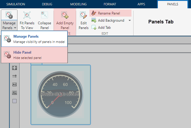
Persistent Panels tab in Simulink Toolstrip

When you add a dashboard panel to a model, the Panels tab appears in the Simulink Toolstrip and shows options for managing and editing panels.

Previously, the Panels tab was only visible when a panel was selected. Starting in R2023a, the Panels tab stays visible when no panel is selected.

If you delete all panels, the Panels tab stays visible while the Simulink model that you are working in is open. If you then close and reopen the model, the Panels tab is no longer visible.

The Panels tab also contains these new options:

• To add an empty panel, on the Panels tab, click Add Empty Panel.

• To rename a panel, on the Panels tab, click Rename Panel. The Parameters tab of the Property Inspector opens. In the Name text box, enter the new panel name.

• To hide a panel, select the panel. Then, on the Panels tab, click Manage Panels and select Hide Panel.

  Note

  To unhide the panel, click the Manage Panels button. In the Manage Panels menu that appears in the lower right corner of the canvas, click the image of the panel.

Callback Button blocks in Dashboard Library and Customizable Blocks Library have same customization options

Starting in R2023a, the Callback Button block from the Dashboard library has the same customization options as the Callback Button block from the Customizable Blocks library. You can change the appearance of the block to look like a real button.

To customize the Callback Button block from the Dashboard library, enter design mode and open the Design tab of the Property Inspector:

1. Select the block.

2. In the Simulink Toolstrip, on the Button tab, click Edit.

3. On the toolbar that appears above the block, click Open Design Tab.

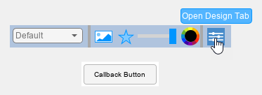
In design mode, you can:

• Upload an image and an icon for each button state.

• Specify the position of the icon relative to the state label.

• Specify the text, color, and position of the label for each button state.

• Upload a foreground or a background image, or set a solid background color.

  The state images are not visible when you set a solid background color. To make the state images visible, in the Property Inspector, on the Design tab, in the Background Image component, turn off Use Background Color.

To configure the state image, icon, label color, and label opacity, use the toolbar above the block.

Use the Design tab in the Property Inspector to:

• Specify the text and position of the label for each button state.

• Specify the icon position.

• Upload a foreground image.

• Upload a background image.

• Set a solid background color.

When you finish editing the design, click the X in the upper-right of the canvas to exit design mode.

Fcn block restored to User-Defined library

The Fcn block has been restored to the Simulink > User-Defined library.

Selector and Assignment blocks support custom integer for index signal

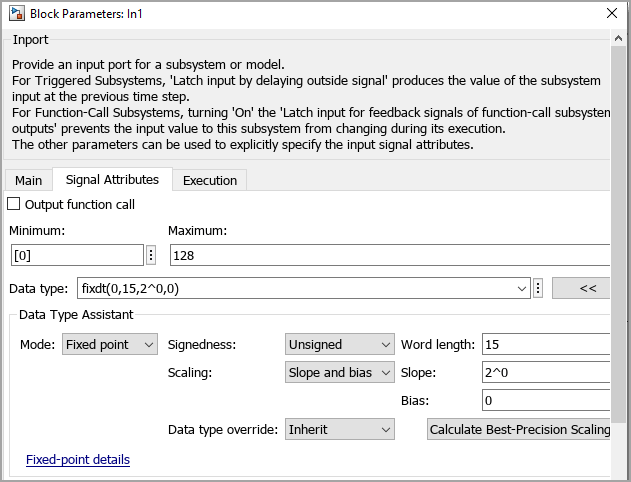
Starting in R2023a, you can specify integer values of custom width (for example,15-bit integer or 23-bit integer) as index signals to the Selector and Assignment blocks. This enhancement allows you to customize your selection of index signal data. When you use Selector and Assignment blocks, you must specify Fixed-point datatype with Word length less than or equal to 128, Slope equal to 1 and Bias equal to 0.

In this example, a 15-bit unsigned integer is used as index signal to the Selector block.

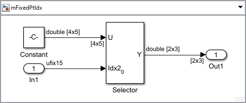
The index signal is configured using the Inport block parameters.

Enhancements to C Caller and C Function blocks and custom code integration

In R2023a, C Caller and C Function blocks and custom code integration have these enhancements.

• C Caller and C Function blocks support using namespaces for types, variables, functions, and classes in your C++ code.

• C Caller and C Function blocks support parameter value implicit casting to specified data type.

• C Function block supports fixed-point data type. You can use the C Function block to:

  • Input signals or parameter values of fixed-point data type, pass them to external C functions, or output them as signals.

  • Process fixed-point data inside the block.

• C Caller block supports global variables in matrix form and structures with a matrix field as input and output.

• When you integrate custom code, you can now use dependent dynamic libraries (DLLs) located in any drive in Windows, including a network drive. With this enhancement, your dependent dynamic library does not have to be in the same drive as your working folder.

Selector block supports variable-size input signal for Index vector(dialog) and Starting index(dialog) index options

Starting in R2023a, when you configure the Selector block for a 1-D variable-size input signal, you can specify the Index Option as Index vector(dialog) or Starting index(dialog). For more information, see Variable-Size Signal Basics.

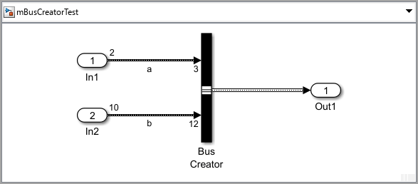
Bus Creator block supports variable-size input signal with upper bound smaller than upper bound of block input port

Starting in R2023a, the Bus Creator block supports variable-size input signals with upper bounds smaller than the upper bound of the corresponding Bus Creator input port. You can configure the upper bound of a Bus Creator input port by specifying the corresponding Simulink.BusElement Dimensions. For more information, see Simulink.BusElement.

In this example, variable-size input signals with upper bounds of 2 and 10 are connected to their corresponding Bus Creator input ports with upper bounds of 3 and 12, respectively.

Parameter Writer block option to skip parameter validation

Starting in R2023a, you can disable parameter validation that occurs during normal mode simulation for Parameter Writer blocks. When parameter validation is disabled for a Parameter Writer block, normal mode simulation of the block is faster.

To locally disable parameter validation for a Parameter Writer block, select the block. Then, in the Property Inspector, clear Validate parameter.

To globally enable or disable parameter validation for Parameter Writer blocks, use the Parameter Writer block validation configuration parameter.

In Bus Element and Out Bus Element block enhancements

Starting in R2023a:

• An Out Bus Element block at the top level of a model lets you specify the name of the top-level bus, signal, or message that appears in a parent subsystem or model.

• The Property Inspector supports In Bus Element and Out Bus Element blocks.

• Warning and error messages for In Bus Element and Out Bus Element blocks now link to the corresponding block in the block diagram, helping you quickly find the source of the warning or error. In previous releases, warning and error messages refer to a hidden block and do not provide a link.

Improved edit shape tool in Graphical Icon Editor

Use the edit tool to edit all supported shapes, for example, rectangles, ellipses, lines, and paths. To edit a shape, select the edit tool and then hover over the shape to view all the edit points forming it. Click an edit point to edit the shape.

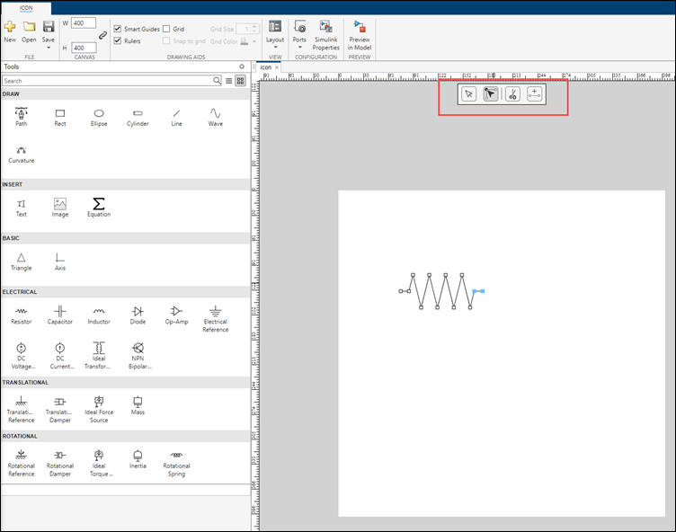
For more information, see Edit the Properties of Block Mask Icon and Its Elements

Plot n-dimensional data in mask look up table control

The mask lookup table control can now plot n-dimensional data. When plotting n-dimensional data, you can:

• Visualize the data in contour, mesh, line, and surface plots.

• Visualize a plot for selected dimensions or slices.

• Select data in the table to highlight corresponding points in the plot.

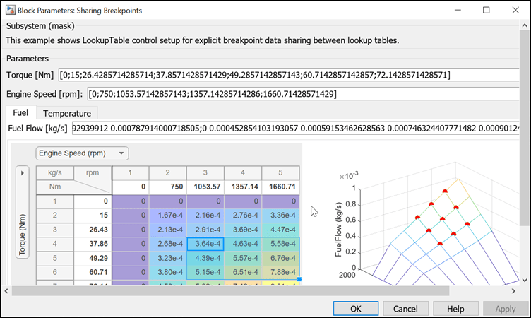
For more information, see Visualize and Plot N-Dimensional Data Using Mask Lookup Table Control

Lookup Table Editor spreadsheet context menu update

The Lookup Table Editor spreadsheet context menu now has a Paste option.

 Functionality being removed or changed

Signal Builder block is not recommended

The Signal Builder block is not recommended. The Signal Builder block has been removed from the Simulink/Sources library. Use the Signal Editor block or other Simulink source blocks instead. Existing models continue to work.

For more information, see Migrate from Signal Builder Block to Signal Editor Block.

Connection to Hardware

Send and Receive data through Nanomsg-Next-Gen (NNG) using NNG Send and NNG Receive blocks

The Raspberry Pi^® Blockset now supports sending and receiving data through NNG on your Raspberry Pi board.

The NNG Send block sends data through NNG using publish and subscribe protocols. The NNG Receive block receives data through NNG using publish and subscribe protocols

Support added for 64-bit Raspberry Pi OS

You can now use the Raspberry Pi Blockset to generate code for the 64-bit Raspberry Pi OS.

To generate code, in the Configuration Parameters dialog box select Hardware Implementation and under Hardware board select Raspberry Pi (64-bit).

Support added for Raspberry Pi Bullseye OS

You can now use the Raspberry Pi Blockset to generate code for the Raspberry Pi Bullseye OS.

BMI160 IMU Sensor block updated to support application interrupts

The BMI160 IMU Sensor in the Raspberry Pi Blockset is updated to support advanced application interrupts. Use the block to generate Single tap, Double tap, High g detection, Any motion, Slow motion, Flat detection, and Data ready interrupts.

MATLAB Function Blocks

Set output variables of any dimension as variable size

You can now set output variables of any dimension to be variable size by clearing the Treat dimensions of length 1 as fixed size property. Prior to R2023a, the MATLAB Function block treated variables with at least one dimension of length 1 as fixed size. This property is enabled by default.

Name-Value Argument Validation: Use arguments blocks inside MATLAB Function blocks

In R2023a, you can use arguments blocks that validate name-value arguments in the MATLAB functions inside MATLAB Function blocks. You declare name-value arguments in an arguments block using dot notation to define the fields of a structure. See Validate Name-Value Arguments.

In this example code snippet, the structure named NameValueArgs defines two name-value arguments, Name1 and Name2. You can use any valid MATLAB identifier for the structure name and the field names.

function result = myFunction(NameValueArgs)
    arguments
        NameValueArgs.Name1
        NameValueArgs.Name2
    end
    ...
end

MATLAB Function blocks support most features of arguments blocks for name-value arguments, including size and class validation, validation functions, and default values. MATLAB Function blocks also support the namedargs2cell function.

MATLAB Function blocks do not support these features of name-value argument validation:

• Name-value input arguments at entry-point functions

• Name-value arguments from class properties using the structName.?ClassName syntax

See Generate Code for arguments Block That Validates Input and Output Arguments.

Output Argument Validation: Use arguments(Output) blocks inside MATLAB Function blocks

In R2023a, you can use arguments blocks that perform output argument validation in the MATLAB functions inside MATLAB Function blocks. Output argument validation declares specific restrictions on function output arguments. Using argument validation, you can constrain the class, size, and other aspects of function output values without writing code in the body of the function to perform these tests.

MATLAB Function blocks support most features of arguments blocks for output variables, including size and class validation, and validation functions. For repeating output arguments, MATLAB Function blocks do not support size validation, class validation, and validation functions.

See Generate Code for arguments Block That Validates Input and Output Arguments.

Input Argument Validation: Use any name for repeating input arguments inside MATLAB Function blocks

In R2023a, in MATLAB Function blocks, you can use any valid MATLAB identifier for the name of a repeating input argument inside an arguments block. MATLAB Function blocks only support a single repeating argument for a function.

In previous releases, MATLAB Function blocks supported only varargin as a repeating input argument.

Grow arrays with end+1 indexing inside MATLAB Function blocks

In R2023a, in MATLAB Function blocks, you can use the end+1 indexing syntax to grow the size of arrays. MATLAB Function blocks support growing arrays in this way either in linear code or in a loop. For example, you can use this code snippet inside MATLAB Function blocks:

...
a = [1 2 3 4 5 6];
a(end+1) = 7;

b = [1 2];
for i = 3:10
    b(end+1) = i;
end
...

To use this functionality, make sure that in the Property Inspector, in Properties > Advanced, the Support variable-size arrays check box is selected.

See Generate Code for Growing Arrays and Cell Arrays with end + 1 Indexing.

Use uint32 enumerations inside MATLAB Function blocks

In R2023a, you can use enumerations that derive from the base type uint32 inside MATLAB Function blocks. For members of uint32 enumerations, MATLAB Function blocks support values that are less than or equal to intmax("int32").

coder.read and coder.write: Read data from .coderdata file into your deployed application

In R2023a, you can use the coder.read function to read data from .coderdata files. In contrast with MAT-files that can be read only inside the MATLAB environment, you can read .coderdata files on any deployment platform that supports a file system. In addition, the .coderdata format supports most primitive and aggregate MATLAB data types, including arrays, structures, and cell arrays. So, the C/C++ code generated for coder.read can be used to read complex aggregate data from .coderdata files into your deployed application.

To export MATLAB data to .coderdata files, use the coder.write function. This function is not supported for code generation.

The code generated for coder.read has two distinct advantages over the code generated for the coder.load function:

• You can update the data stored in .coderdata files without having to regenerate code, as long as the type and size of the new data matches those of the old data.

• The data is not hard-coded in the generated code, thereby improving the readability of the generated code.

This is an example workflow that uses the coder.read and coder.write functions:

1. Use the coder.write (MATLAB Coder) function at the MATLAB command line to store the data in .coderdata files. For example, create a file named myfile.coderdata by using these commands:

   c = rand(100);
   coder.write('myfile.coderdata',c);

   Wrote file 'myfile.coderdata'. You can read this file with 'coder.read'.

2. In your MATLAB Function block, use the coder.read (MATLAB Coder) function to read data from the .coderdata files. For example:

   function y = fcn(x) %#codegen
   dataOut = coder.read('myfile.coderdata');
   y = x + mean(dataOut,"all");
   end
   

3. Add input and display blocks. Pass input 1 to the MATLAB Function block and run the simulation.

   

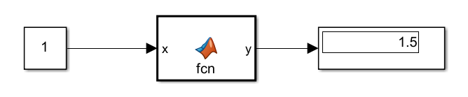
4. You can now update the data stored in myfile.coderdata to a different 100-by-100 array of double type. If you run simulation again, the model now reads and uses the new data.

   d = rand(100) - 1;
   coder.write('myfile.coderdata',d);
   

   

For more information and examples, see coder.read, coder.write, and Data Read and Write Considerations (MATLAB Coder).

Code generation for more MATLAB functions

• cd

• filesep

• griddedInterpolant

• inedges

• isfile

• isfolder

• ismac

• ispc

• isuniform

• isunix

• mape

• mustBeFile

• mustBeFolder

• mustBeInRange

• namedargs2cell

• NET.isNETSupported

• num2cell

• outedges

• pathsep

• polyshape

• predecessors

• pwd

• rmse

• strcat

• successors

• warning

Code generation for more toolbox functions

In R2023a, you can generate code for many additional toolbox functions and objects. For a list of all functions and objects that are supported for code generation, see:

• Functions and Objects Supported for C/C++ Code Generation (Category List)

• Functions and Objects Supported for C/C++ Code Generation (Alphabetical List)

These are links to the release notes of some toolboxes that added code generation support in R2023a:

Computer Vision Toolbox

See Generate C and C++ Code Using MATLAB Coder: Support for functions (Computer Vision Toolbox).

Image Processing Toolbox

See C Code Generation: Generate code from additional functions using MATLAB Coder (Image Processing Toolbox).

Signal Processing Toolbox

See C/C++ Code Generation Support: Code generation for digital filter design, multirate signal processing, and waveform generation (Signal Processing Toolbox).

Statistics and Machine Learning Toolbox

See Generate C/C++ code for prediction using Gaussian kernel classification and regression models (requires MATLAB Coder) (Statistics and Machine Learning Toolbox).

Wavelet Toolbox

See C/C++ Code Generation: Automatically generate code for wavelet functions (Wavelet Toolbox).

Modeling Guidelines

Updates to modeling guidelines for code generation

Guideline for timer service interface in component deployment modeling

You can use guideline cgsl_0410: Timer service for component deployment to model export-function and single-rate, rate-based models that generate entry-point functions. You can configure and generate timer service interface code for:

• Aperiodic exported functions generated from models that rely on elapsed time values (by using Discrete Time Integrator and Weighted Sample Time blocks).

• Periodic entry-point functions generated from models that use blocks that rely on absolute time values (such as Sine Wave and Pulse Generator blocks).

• Periodic entry-point functions generated from models that use blocks that rely on the elapsed time value in an aperiodic context.

Within a model, you represent requests for a clock tick implicitly when you use blocks that rely on a time value. For these blocks, depending on the context, the code generator assumes that the clock resolution is the sample period of the function or fixed-step size (fundamental sample time) of the model.

For more information about the timer service interface, see Generate C Timer Service Interface Code for Component Deployment (Embedded Coder).

Removal of code generation modeling guidelines

Starting in R2023a, these code generation modeling guidelines are removed.

Modeling Guideline	Rationale
cgsl_0104: Modeling global shared memory using data stores	Inconsistent with modeling by using a service interface. Conflicts with modeling guideline hisl_0013: Usage of data store memory
cgsl_0105: Modeling local shared memory using data stores	Inconsistent with modeling by using a service interface. Conflicts with modeling guideline hisl_0013: Usage of data store memory
cgsl_0205: Signal handling for multirate models	Redundant. Use hisl_0042: Configuration Parameters > Solver > Tasking and sample time options
cgsl_0206: Data integrity and determinism in multitasking models	Redundant. Use hisl_0042: Configuration Parameters > Solver > Tasking and sample time options
cgsl_0302: Diagnostic settings for multirate and multitasking models	Redundant. To verify the configuration parameters, use: hisl_0044: Configuration Parameters > Diagnostics > Sample Time hisl_0303: Configuration Parameters > Diagnostics > Data Validity > Merge blocks hisl_0013: Usage of data store memory

Guideline for check safety-related diagnostic settings for Stateflow

Starting in R2023a, the guideline "hisl_0311: Configuration Parameters > Diagnostics > Stateflow" no longer recommends that the configuration parameter Use of machine-parented data instead of Data Store Memory is set to none or warning because the configuration parameter has been removed. For information on the guideline, see hisl_0311: Configuration Parameters > Diagnostics > Stateflow.

Note that the configuration parameter was removed because Stateflow charts no longer support machine-parented data. You can check for machine-parented data and use the Upgrade Advisor to convert machine-parented data to chart-parented data store memory. For more information, see Consult the Upgrade Advisor and Check for machine-parented data.