Linearize at Trimmed Operating Point
This example shows how to linearize a model at a trimmed steady-state operating point (equilibrium operating point) using the Model Linearizer.
The operating point is trimmed by specifying constraints on the operating point values, and performing an optimization search that meets these state and input value specifications.
Open the Simulink® model.
openExample("magball")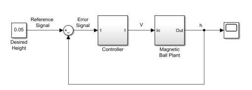
Open Model Linearizer for the model.
In the Simulink model window, in the Apps gallery, click Model Linearizer.
To specify linearization input and output points, open the Linearization tab. To do so, in the Apps gallery, click Linearization Manager.
To specify an analysis point for a signal, click the signal in the model. Then, on the Linearization tab, in the Insert Analysis Points gallery, select the type of analysis point.
Configure the output signal of the Controller block as an Input Perturbation.
Configure the output signal of the Magnetic Ball Plant block as an Open-loop Output.
Annotations appear in the model indicating which signals are designated as analysis points.
Tip
Alternatively, if you do not want to introduce changes to the Simulink model, you can specify the analysis points in Model Linearizer. For more information, see Specify Portion of Model to Linearize in Model Linearizer.
Create a new steady-state operating point at which to linearize the model. In Model Linearizer, in the Operating Point drop-down list, select Trim model.

In the Trim the model dialog box, the Specifications tab shows the default specifications for model trimming. By default, all model states are specified to be at equilibrium, indicated by the check marks in the Steady State column.
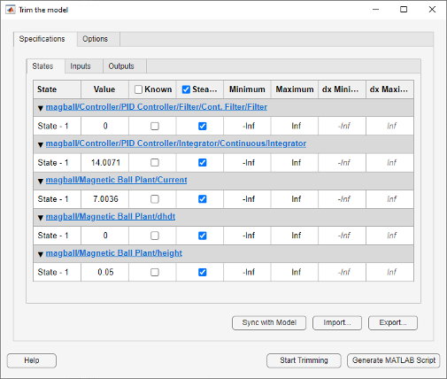
Specify a steady-state operating point at which the magnetic ball height remains fixed at the reference signal value, 0.05. In the States tab, select Known for the height state. This selection tells Model Linearizer to find an operating point at which this state value is fixed.

Since the ball height is greater than zero, the current must also be greater than zero. Enter
0for the minimum bound of the Current block state.
Compute the operating point.
Click
 Start trimming.
A new variable,
op_trim1, appears in the Linear Analysis Workspace.
In the Operating Point drop-down list, this operating point is now selected as the operating point to be used for linearization.
Linearize the model at the specified operating point and generate a bode plot of the result. Click
 Bode. The Bode plot of the linearized plant appears, and the
linearized plant
Bode. The Bode plot of the linearized plant appears, and the
linearized plant linsys1appears in the Linear Analysis Workspace.
Tip
Instead of a Bode plot, generate other response types by clicking the corresponding button in the plot gallery.
Right-click on the plot and select information from the Characteristics menu to examine characteristics of the linearized response.