Deployment
Generate C/C++ code and deploy pretrained XGBoost models (requires MATLAB Coder)
You can generate C/C++ code and perform inference using pretrained XGBoost models.
Save a CompactClassificationXGBoost or CompactRegressionXGBoost model object by using saveLearnerForCoder, and then load the model in the entry-point
function for code generation by using loadLearnerForCoder.
Anomaly Detection Blocks: Find anomalies in data and generate code in Simulink
You can integrate the isanomaly function of isolation forest objects and isanomaly function of the one-class SVM objects into Simulink® using the new anomaly detector blocks. Import a trained anomaly
detection model and configure data types using the Block Parameters dialog
box.
Isolation Forest Anomaly Detector — This block finds anomalies in new data using a trained isolation forest model object (
IsolationForest).One-Class SVM Anomaly Detector — This block finds anomalies in new data using a trained one-class support vector machine (SVM) model object (
OneClassSVM).
The blocks support C/C++ code generation and fixed-point conversion. You can generate C and C++ code using Simulink Coder™, and design and simulate fixed-point systems using Fixed-Point Designer™.
Override model properties in the IncrementalClassificationNaiveBayes Predict Block
You can override model properties such as Cost,
Prior, and ScoreTransform in the
IncrementalClassificationNaiveBayes Predict block using the Block
Parameters dialog box. In previous releases, you set these properties when creating
the initial incrementalClassificationNaiveBayes model object.
ClassificationECOC Predict block: Use machine learning models trained with binary kernel learners
The ClassificationECOC
Predict block now supports ClassificationECOC and CompactClassificationECOC machine learning models trained with binary
kernel learners.
Generate C/C++ code for performing incremental learning using kernel classification and regression functions (requires MATLAB Coder)
You can generate C/C++ code that trains a kernel classification or regression
model in real time, as batches of observations become available. You can save an
incrementalClassificationKernel or incrementalRegressionKernel model by using saveLearnerForCoder, and then load the model in the entry-point
function for code generation by using loadLearnerForCoder (see Introduction to Code Generation for Statistics and Machine Learning Functions). These incremental learning functions
support code generation:
The
fitfunction fits the model to incoming data by updating the coefficients.The
predictfunction predicts responses given incoming data.The
lossfunction returns the classification or regression loss of the model for incoming data.The
updateMetricsfunction updates performance metrics given incoming data.The
updateMetricsAndFitfunction updates performance metrics and fits the model to incoming data.
Generate C/C++ code for performing incremental learning using a multiclass classification model with kernel binary learners (requires MATLAB Coder)
You can generate C/C++ code for incrementalClassificationECOC model objects that use kernel binary
learners. For more information, see Extended Capabilities and Introduction to Code Generation for Statistics and Machine Learning Functions.
saveLearnerForCoder Function: Specify kernel computation
method for Gaussian SVM and ECOC models
If your trained model is a Gaussian SVM model, or an ECOC model with at least one
Gaussian SVM binary learner, you can specify
OptimizeKernelFor=ComputationMethod in saveLearnerForCoder to select the kernel computation method to use
in the generated C/C++ code. When you specify
OptimizeKernelFor="speed" (the default), the SVM model uses
an expansion formulation for fast calculations of the Gram matrix. In some cases,
such as when your trained model has a small kernel scale, this formulation might
lead to numerical precision loss. To use an exact formulation for the calculations,
specify OptimizeKernelFor="accuracy". This
setting typically results in slower calculations.
Multithreading support for C/C++ code generation of ensembles of trees and ensembles of discriminant analysis models (requires MATLAB Coder)
When you generate single- or double-precision
C/C++ code for ensembles consisting of all tree learners or all discriminant
analysis learners, the generated code of the predict object
function now uses parfor to create loops that run in
parallel on supported shared-memory multicore platforms. For more information, see
Code Generation (for classification) and Code Generation (for
regression).
Apps
Machine Learning Apps: Import a trained model from the MATLAB workspace
Import a supported trained machine learning model from the MATLAB® workspace into Classification Learner and Regression Learner in one of two ways:
On the Learn tab, in the File section, select New Session > From Trained Model.
On the Learn tab, in the File section, click Import Model.
After you import a trained model into the app, you can:
Assess model performance using a test data set.
Explain model behavior using interpretability plots.
Export the model for deployment.
For a list of supported models and restrictions, see Import Trained Model from Workspace into Classification Learner or Regression Learner.
Machine Learning Apps: Train customizable neural networks (requires Deep Learning Toolbox)
Create a customizable neural network model in Classification Learner or Regression Learner by selecting the model preset Fully Connected Customizable Neural Network or Residual Customizable Neural Network in the Models section of the Learn tab. To customize the model's neural network architecture, select the model in the models pane, and click Customize Network on the model Summary tab. The default model for the fully connected customizable network contains five fully connected layers (excluding the final fully connected layer for prediction). The default model for the residual customizable network contains one residual connection. For more information, see Customizable Neural Network Models and Edit Customizable Neural Network Using Network Editor in Classification Learner or Regression Learner.
Machine Learning Apps: Specify validation and test partitions at MATLAB command line
When you launch Classification Learner or Regression Learner from the MATLAB command line, use the ValidationPartition
name-value argument to specify a cvpartition object that defines the validation scheme and the
indexing for the validation sets. To define the indexing for the test data set,
specify a cvpartition object using the
TestPartition name-value argument. For more information,
see Classification Learner and Regression Learner.
Machine Learning Apps: Export partitions and data sets
Export the partitions used to compute validation and test metrics, as well as the data sets, from the current session to the MATLAB workspace. In the Export section of the Learn tab, select Export > Export Partitions and Data Sets. For more information, see Export Partitions and Data Sets from Classification Learner or Regression Learner.
Machine Learning Apps: Export a feature ranking plot
Export a feature ranking plot or its data by first creating the plot using the Feature Selection button in the Options section of the Learn tab. Select Export Plot to Figure or Export Plot Data in the Export section.
Functionality being removed or changed
Machine Learning Apps: Automatically select the number of predictors to sample in ensemble tree models
Behavior change
In Classification Learner and Regression Learner, when you create a draft tree
model from the Ensemble Classifiers or Ensembles
of Trees section of the Models gallery, the
default setting for the number of predictors to sample is now
Auto. For Boosted Tree and RUSBoosted Tree models,
Auto is equivalent to the default Select
All setting in previous releases. For Bagged Tree models,
Auto sets the number of predictors to sample as the
square root of the number of predictors in Classification Learner, and one third
of the number of predictors in Regression Learner.
Machine Learning
Build, share, and deploy machine learning workflows using machine learning pipelines
A machine learning pipeline is a set of connected steps, called components, that are executed in a specified order to process data and perform machine learning. You can use pipelines to develop, share, and deploy end-to-end machine learning workflows.
Use the built-in components for data processing, feature selection, and supervised learning, or convert your custom functions into pipeline components. You can combine components to create pipelines for various machine learning applications.
For an example of a pipelines workflow, see Create Simple Classification Pipeline. For more information about the available components and functionality, see Machine Learning Pipelines.
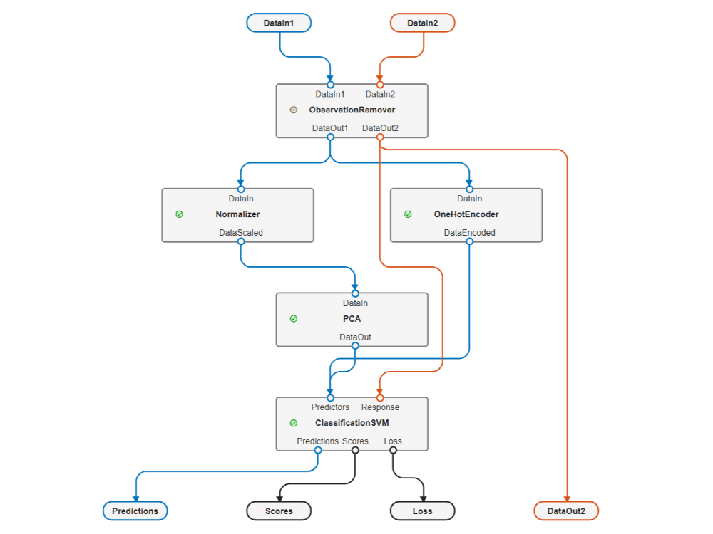
Build, share, and deploy machine learning workflows using machine learning pipelines
UMAP: Reduce and visualize high-dimensional data
Using the umap
function, you can reduce high-dimensional data to a low-dimensional embedding in
order to view natural clustering and perform exploratory data analysis. For details,
see the function reference page.
Evaluate model performance on slices of data
Evaluate the performance of a model on subsets of data (data slices) by using the
sliceMetrics function. The function creates a
sliceMetrics object, which you can use to compute metrics (such
as accuracy or mean squared error) on the data slices and their complements. Use the
report
object function to summarize the metrics in a table, and use the plot
object function to visualize the metrics as bar graphs.
Synthetic Data Generation: Generate synthetic data for imbalanced data sets using SMOTE
You can use the synthetic minority oversampling technique (SMOTE) algorithm to generate synthetic data for binary classification. Using SMOTE can be helpful when you have imbalanced data, that is, when one class contains many more observations than the other.
Use the
synthesizeTabularDatafunction withMethod="smote".Alternatively, create a
smoteTabularSynthesizerobject, and then use thesynthesizeTabularDataobject function.
Regardless of the method used (SMOTE or binning), the
synthesizeTabularData functions can return synthetic
observations for one or two classes.
XGBoost Importer: Perform inference using imported XGBoost models
Import pretrained XGBoost regression and classification models into MATLAB and perform inference using the new importModelFromXGBoost function.
Classification — Import binary and multiclass classification models as
CompactClassificationXGBoostobjects.Regression — Import regression models as
CompactRegressionXGBoostobjects.
Incremental Learning: Create a model for incremental normalization
The incrementalNormalizer function creates a model object that is
suitable for incremental normalization. Unlike the zscore function, for which you must provide all of the data before
computing z-scores, incrementalNormalizer
allows you to update the weighted predictor mean and standard deviation estimates
incrementally and return z-scores by supplying chunks of data to
the incremental fit
function.
You can create the following types of incremental normalization model objects:
ZScoreNormalizer— Use simple weighting.ExponentiallyWeightedNormalizer— Assign higher weights to newer observations.ClassWeightedNormalizer— Assign weights by individual class.
After creating a model object, you can train the model and calculate z-scores in real time as the model accesses data, either per individual observation or specified batch size.
The
fitfunction updates the model object with information computed from the input model and data. The function optionally returns the z-scores.The
transformfunction transforms the input data into z-scores by using the incremental normalizer model.The
resetfunction resets all learned parameters of the model.
Generate counterfactual examples to better understand binary classifier decisions
Gain insight into binary classifier decisions by generating counterfactual
examples using the counterfactuals function. Counterfactual examples identify the
minimal modifications needed to change the predicted label of a given
observation.
Quantile Regression: Perform hyperparameter optimization with multiple quantiles
You can optimize the hyperparameters of a quantile regression model with multiple
quantiles. Specify the OptimizeHyperparameters and
Quantiles name-value arguments in the call to fitrqlinear or fitrqnet.
If you perform Bayesian hyperparameter optimization when creating a RegressionQuantileLinear or RegressionQuantileNeuralNetwork object, the
HyperparameterOptimizationResults property contains a
SupervisedLearningBayesianOptimization object. In previous
releases, the stored object is a BayesianOptimization object.
Hyperparameter Optimization: Perform cost-sensitive hyperparameter optimization for classification models
You can optimize classification model hyperparameters with respect to
misclassification cost. When you use a classification fit function, specify the
OptimizeHyperparameters and
HyperparameterOptimizationOptions name-value arguments. In
the HyperparameterOptimizationOptions structure or object, set
the LossFun value to "classifcost",
"mincost", or "auto-cost", depending on
the classification fit function.
Depending on the type of supervised learning fit function you use to perform
hyperparameter optimization, you can set the LossFun value to
"auto-cost", "classifcost",
"classiferror", "mincost",
"mse", or "quantile".
GPU Support: Specify GPU arrays for cvpartition (requires
Parallel Computing Toolbox)
You can now partition data for cross-validation on a GPU by supplying GPU array
stratification variables or custom test sets to the cvpartition function. The object functions repartition, summary, test, and training accept the resulting cvpartition
object and can execute on a GPU.
For a full list of Statistics and Machine Learning Toolbox™ functions that accept GPU arrays, see Function List (GPU Arrays).
GPU Support: Specify GPU arrays for Gaussian process regression models (requires Parallel Computing Toolbox)
The following functions now support GPU arrays, enabling you to execute the functions on a GPU:
The
fitrgpfunction accepts GPU array input arguments.Most object functions of the models
RegressionGP,CompactRegressionGP, andRegressionPartitionedGPnow support GPU array input arguments. The functions that do not arelimeandshapley.
For a full list of Statistics and Machine Learning Toolbox functions that accept GPU arrays, see Function List (GPU Arrays).
GPU Support: fitcecoc supports kernel learners for
gpuArray inputs (requires Parallel Computing Toolbox)
You can specify kernel learners when you create a CompactClassificationECOC or ClassificationPartitionedKernelECOC model object by passing
gpuArray data to fitcecoc.
To view the limitations of this support, see the Extended Capabilities sections in
the documentation for fitcecoc,
CompactClassificationECOC, and
ClassificationPartitionedKernelECOC.
GPU Support: Specify GPU arrays when computing Shapley values using the Linear SHAP algorithm (requires Parallel Computing Toolbox)
The shapley
and fit
functions accept GPU array input arguments when the machine learning model is a
regression or binary classification linear model listed below, and the function uses
an interventional algorithm (Method="interventional").
The supported models are:
RegressionSVM,CompactRegressionSVM,ClassificationSVM, andCompactClassificationSVMmodels that use a linear kernel function
Performing Shapley value computations on a GPU is typically faster than on a CPU
when you have a large number of query points and you do not specify an output
function (OutputFcn=[]).
Neural Networks: Specify custom neural network architecture for data with categorical predictors
Specify a custom neural network architecture for categorical predictors using the
Network
argument of the fitcnet
and fitrnet
functions. Specify the neural network architecture as an array of deep learning
layers or as a dlnetwork object. Use this
argument when the fitcnet and fitrnet
functions do not provide the neural network architecture that you need for your task
such as neural networks with skip-connections.
Neural Networks: Convergence information and training history for custom neural network architectures
For ClassificationNeuralNetwork and RegressionNeuralNetwork objects fit using a dlnetwork or layer array that
specifies the neural network architecture:
The
ConvergenceInfoproperty now contains values for theValidationChecksfield.The
TrainingHistoryproperty now contains theValidationChecksandTimevariables.
fitrnet Function: Use validation data when the regression
model has multiple response variables
When creating a neural network regression model with multiple response variables,
you can use validation data by specifying the ValidationData value in the call to fitrnet. For further customization, you can also specify the ValidationFrequency and ValidationPatience name-value arguments.
Categorical Predictors: Count the number of predictors in tabular data after encoding the categorical variables
Count the number of predictors in tabular data after encoding the categorical
variables using the countPredictorsAfterCategoricalEncoding function.
You can use this function to help define custom neural network architectures for
the fitcnet
and fitrnet
functions.
sequentialfs Function: Compute the criterion value for each
candidate feature set in parallel (requires Parallel Computing Toolbox)
Compute the criterion value for each candidate feature set in parallel when no
cross-validation is performed. In previous releases, sequentialfs performs only cross-validation in parallel. That is,
the function runs computations in parallel when both of the following are true:
Starting with this release, provided that UseParallel=true in
the options structure, the function computes the criterion value for each candidate
feature set in parallel when no cross-validation is requested or when
cross-validation is requested with one Monte Carlo repetition.
Example of handling class imbalance in binary classification
A new example, Handle Class Imbalance in Binary Classification, shows how to handle class imbalance in binary classification using decision thresholding, random undersampling, random oversampling, and SMOTE (Synthetic Minority Oversampling Technique).
Functionality being removed or changed
Hyperparameter Optimization: Store Bayesian optimization results in a new object when using a supervised learning fit function
Behavior change
If you perform Bayesian hyperparameter optimization by using a supervised
learning fit function, the optimization results are stored in a
SupervisedLearningBayesianOptimization object. In previous
releases, the optimization results are stored in a BayesianOptimization object.
A cross-validated neural network classification model is a
ClassificationPartitionedNeuralNetwork object
Behavior change
A cross-validated neural network classification model is a ClassificationPartitionedNeuralNetwork object. In previous
releases, a cross-validated neural network classification model is a ClassificationPartitionedModel
object.
You can create a ClassificationPartitionedNeuralNetwork
object in two ways:
Create a cross-validated model from a neural network classification model
ClassificationNeuralNetworkby using thecrossvalfunction.Create a cross-validated model by using the
fitcnetfunction and specifying one of the name-value argumentsCrossVal,CVPartition,Holdout,KFold, orLeaveout.
A cross-validated quantile neural network regression model is a
RegressionPartitionedQuantileNeuralNetwork object
Behavior change
A cross-validated quantile neural network regression model is a RegressionPartitionedQuantileNeuralNetwork object. In previous
releases, a cross-validated quantile neural network regression model is a
RegressionPartitionedQuantileModel object.
You can create a RegressionPartitionedQuantileNeuralNetwork
object in two ways:
Create a cross-validated model from a quantile neural network regression model
RegressionQuantileNeuralNetworkby using thecrossvalfunction.Create a cross-validated model by using the
fitrqnetfunction and specifying one of the name-value argumentsCrossVal,CVPartition,Holdout,KFold, orLeaveout.
rocmetrics and perfcurve Functions:
Compute performance curves when a positive class is missing
Behavior change
You can now compute performance curves using rocmetrics or perfcurve when a positive class is
missing from the true class labels. For example, each function can return
metrics when a particular class appears in the training data but not in the
validation or test data. Some returned metrics might have NaN
values.
Statistics
Design of Experiments: Create a fractionalFactorialDOE object to
generate an experiment design
Generate a two-level fractional factorial experiment design by using the fractionalFactorialDOE function to create an object of the same name.
The object properties include information about the design, model, and factors used
to generate the design. After creating the object, you can use the fitlm function to fit a linear model to the design points. Use the
fractionalFactorialTypes function to return a table containing the
resolution level and maximum number of runs for all possible two-level fractional
factorial design types for both a set of factors and an experiment model.
Analysis of Lifetime Data: Create an accelerated life testing model
Create an AcceleratedLifeModel model object for accelerated life testing by
using the fitacclife function. The function fits an accelerated life model to
input data that contains stressor levels and their corresponding failure times.
After creating the object, you can use it to generate plots and compute mean failure
times, distribution functions, and failure time probabilities at specific stressor levels.
Compute distribution functions using the
distfcnandicdffunctions, and create distribution plots with thedistplotfunction.Compute and plot mean failure times at stressor levels using the
meanfailtimeandmeanfailplotfunctions.Plot predicted failure time probabilities at stressor levels using the
probplotfunction.Compute failure time acceleration factors at stressor levels relative to a baseline stressor level using the
accelfactorfunction.Compute confidence intervals for the fitted model coefficients using the
coefcifunction.
Linear Regression: Find a minimum or maximum response value and calculate predictor values that yield a specified response (requires Optimization Toolbox)
Two new object functions are available for LinearModel and CompactLinearModel objects:
optimizeResponse: Use this function to find a minimum or maximum response value for a linear regression model and the predictor values for that response value (additionally requires Global Optimization Toolbox if the model includes interaction terms with categorical predictors whose values are not fixed usingCategoricalValues).matchResponse: Use this function to calculate the predictor values that correspond to a specified response value and have the smallest response variance (additionally requires Global Optimization Toolbox if the model includes categorical predictors whose values are not fixed usingCategoricalValues).
GPU Support: Specify GPU arrays for noncentral chi-square distribution (requires Parallel Computing Toolbox)
The ncx2cdf, ncx2pdf, ncx2inv, and ncx2stat functions now support GPU arrays, enabling you to execute
them on a GPU.
For a full list of Statistics and Machine Learning Toolbox functions that accept GPU arrays, see Function List (GPU Arrays).
GPU Support: Specify GPU arrays for Rician distribution (requires Parallel Computing Toolbox)
The fitdist and mle functions now support GPU arrays for Rician
distributions.
For a full list of Statistics and Machine Learning Toolbox functions that accept GPU arrays, see Function List (GPU Arrays).
mhsample Function: For improved performance, explicitly
specify Gaussian or Student's t proposal distribution
The Proposal name-value argument enables you to explicitly
specify the distributions in this table by their name. You can tune the sampler by
adjusting corresponding distribution parameters using name-value argument
syntax.
| Name | Proposal Distribution | Parameters |
|---|---|---|
"Gaussian" | Multivariate Gaussian distribution |
|
"t" | Multivariate Student's t distribution |
|
When you specify these distributions by setting Proposal
instead of setting the PropPDF or LogPropPDF
to a custom function handle to either of these distributions,
mhsample might show improved performance. For example, the
code below compares the run-time performance of mhsample when
implicitly specifying a scale 1 Gaussian proposal distribution by using a custom
function and when explicitly specifying a scale 1 Gaussian proposal by using the
Proposal and Scale name-value
arguments. The mhsample function is 20x faster when a Gaussian
proposal is explicitly specified.
F  = @(x) -x.^2 + log(2 + sin(5*x) + sin(2*x)); % Target stationary distribution log-PDF
numSamples = 500000;                            % Length of the MCMC chain
propPDF = @(x,y)mvnpdf(x,y,1);                  % Proposal probability density function
propRNG = @(x)mvnrnd(x,1);                      % Proposal random number generator

% Implicitly specify Gaussian proposal by specifying a function handle
% to Gaussian random number generator
rng(1,"twister")
timeitimplicit = @()mhsample(0,numSamples,LogPDF=F,PropPDF=propPDF, ...
    PropRND=propRNG,Symmetric=true);
timecgp = timeit(timeitimplicit);

% Explicitly specify Gaussian proposal, under the same conditions, by naming
% the proposal distribution using Proposal.
rng(1,"twister")
timeitexplicit = @()mhsample(0,numSamples,LogPDF=F,Proposal="Gaussian", ...
    Scale=1);
timegp = timeit(timeitexplicit);
Functionality being removed or changed
mhsample Function: NumChains
name-value argument replaces nchains
Behavior change
When you call mhsample, to specify the number
of Markov chains to generate from the Metropolis-Hasting algorithm, use the
NumChains name-value argument instead of
nchains. Although you should update your code to use
NumChains instead of nchains, there
are no plans to remove nchains.
Visualization
controlchart Function: Create P', NP', U', and C'
charts
The controlchart function can now plot
Laney P', NP', U', and C' charts, which adjust the control limits for subgroup sizes
and inter-subgroup variations.
confusionchart Function: Customize confusion chart
display
You can now customize the rotation of row (y-axis) and column (x-axis) labels of
ConfusionMatrixChart objects:
Specify the rotation of the row and column labels using the
RowTickLabelRotationandColumnTickLabelRotationproperties.Prevent row and column labels from automatically rotating when you resize a confusion chart by specifying the
RowTickLabelRotationModeandColumnTickLabelRotationModeproperties.
You can also specify to display zero values in the chart using the ZerosVisible property.
To create a confusion chart, use the confusionchart function. For more information about how to set these
properties, see ConfusionMatrixChart Properties.
Functionality being removed or changed
controlchart Function: Set the center line value when
specifying Limits and Rules
Behavior change
When you specify both the Limits and
Rules name-value arguments for controlchart, the center line
value is equal to the middle element value of Limits. In
previous releases, the center line value is equal to the arithmetic mean of all
measurement values.