Solve DAEs Using Mass Matrix Solvers

Solve differential algebraic equations by using one of the mass matrix solvers available in MATLAB®. To use this workflow, first complete steps 1, 2, and 3 from Solve Differential Algebraic Equations (DAEs). Then, use a mass matrix solver instead of ode15i.

This example demonstrates the use of ode15s or ode23t. For details on the other solvers, see Choose an ODE Solver and adapt the workflow on this page.

Step 1. Convert DAEs to Function Handles

The code from steps 1 to 3 of Solve Differential Algebraic Equations (DAEs) is:

syms x(t) y(t) T(t) m r g
eqn1 = m*diff(x(t), 2) == T(t)/r*x(t);
eqn2 = m*diff(y(t), 2) == T(t)/r*y(t) - m*g;
eqn3 = x(t)^2 + y(t)^2 == r^2;
eqns = [eqn1 eqn2 eqn3];
vars = [x(t); y(t); T(t)];
origVars = length(vars);
[eqns,vars] = reduceDifferentialOrder(eqns,vars);
[DAEs,DAEvars] = reduceDAEIndex(eqns,vars);
[DAEs,DAEvars] = reduceRedundancies(DAEs,DAEvars);

From the output of reduceDAEIndex and reduceRedundancies, you have a vector of equations DAEs and a vector of variables DAEvars. To use ode15s or ode23t, you need two function handles: one representing the mass matrix of a DAE system, and the other representing the right sides of the mass matrix equations. These function handles form the equivalent mass matrix representation of the ODE system where $\mathit{M}\left(\mathit{t},\mathit{y}\left(\mathit{t}\right)\right){\mathit{y}}^{\prime }\left(\mathit{t}\right)=\mathit{f}\left(\mathit{t},\mathit{y}\left(\mathit{t}\right)\right)$.

Find these function handles by using massMatrixForm to get the mass matrix M and the right sides F.

[M,f] = massMatrixForm(DAEs,DAEvars)

M = 
$$\left(\begin{array}{ccccccc}0& 0& 0& 0& 0& 0& 0\\ 0& 0& 0& 0& 0& 0& 0\\ 0& 0& 0& 0& 0& 0& 0\\ 0& 0& 0& 0& 0& 0& 0\\ 0& 0& 0& 0& 0& 0& 0\\ 0& 0& 0& 0& -1& 0& 0\\ 0& -1& 0& 0& 0& 0& 0\end{array}\right)$$

f = 
$$\left(\begin{array}{c}\frac{T\left(t\right)\hspace{0.17em}x\left(t\right)-m\hspace{0.17em}r\hspace{0.17em}\mathrm{Dxtt}\left(t\right)}{r}\\ -\frac{g\hspace{0.17em}m\hspace{0.17em}r-T\left(t\right)\hspace{0.17em}y\left(t\right)+m\hspace{0.17em}r\hspace{0.17em}\mathrm{Dytt}\left(t\right)}{r}\\ r^2-{x\left(t\right)}^2-{y\left(t\right)}^2\\ -2\hspace{0.17em}\mathrm{Dxt}\left(t\right)\hspace{0.17em}x\left(t\right)-2\hspace{0.17em}\mathrm{Dyt}\left(t\right)\hspace{0.17em}y\left(t\right)\\ -2\hspace{0.17em}{\mathrm{Dxt}\left(t\right)}^2-2\hspace{0.17em}{\mathrm{Dyt}\left(t\right)}^2-2\hspace{0.17em}\mathrm{Dxtt}\left(t\right)\hspace{0.17em}x\left(t\right)-2\hspace{0.17em}\mathrm{Dytt}\left(t\right)\hspace{0.17em}y\left(t\right)\\ -\mathrm{Dytt}\left(t\right)\\ -\mathrm{Dyt}\left(t\right)\end{array}\right)$$

The equations in DAEs can contain symbolic parameters that are not specified in the vector of variables DAEvars. Find these parameters by using setdiff on the output of symvar from DAEs and DAEvars.

pDAEs = symvar(DAEs);
pDAEvars = symvar(DAEvars);
extraParams = setdiff(pDAEs,pDAEvars)

extraParams = $$\left(\begin{array}{ccc}g& m& r\end{array}\right)$$

The mass matrix M does not have these extra parameters. Therefore, convert M directly to a function handle by using odeFunction.

M = odeFunction(M,DAEvars);

Convert f to a function handle. Specify the extra parameters as additional inputs to odeFunction.

f = odeFunction(f,DAEvars,g,m,r);

The rest of the workflow is purely numerical. Set parameter values and create the function handle.

gVal = 9.81;
mVal = 1;
rVal = 1;
F = @(t,Y) f(t,Y,gVal,mVal,rVal);

Step 2. Find Initial Conditions

The solvers require initial values for all variables in the function handle. Find initial values that satisfy the equations by using the MATLAB decic function. The decic accepts guesses (which might not satisfy the equations) for the initial conditions, and tries to find satisfactory initial conditions using those guesses. decic can fail, in which case you must manually supply consistent initial values for your problem.

First, check the variables in DAEvars.

DAEvars

DAEvars = 
$$\left(\begin{array}{c}x\left(t\right)\\ y\left(t\right)\\ T\left(t\right)\\ \mathrm{Dxt}\left(t\right)\\ \mathrm{Dyt}\left(t\right)\\ \mathrm{Dytt}\left(t\right)\\ \mathrm{Dxtt}\left(t\right)\end{array}\right)$$

Here, Dxt(t) is the first derivative of x(t), Dytt(t) is the second derivative of y(t), and so on. There are 7 variables in a 7-by-1 vector. Thus, guesses for initial values of variables and their derivatives must also be 7-by-1 vectors.

Assume the initial angular displacement of the pendulum is 30° or pi/6, and the origin of the coordinates is at the suspension point of the pendulum. Given that we used a radius rVal of 1, the initial horizontal position x(t) is rVal*sin(pi/6). The initial vertical position y(t) is -rVal*cos(pi/6). Specify these initial values of the variables in the vector y0est.

Arbitrarily set the initial values of the remaining variables and their derivatives to 0. These are not good guesses. However, they suffice for our problem. In your problem, if decic errors, then provide better guesses and refer to the decic page.

y0est = [rVal*sin(pi/6); -rVal*cos(pi/6); 0; 0; 0; 0; 0];
yp0est = zeros(7,1);

Create an option set that contains the mass matrix M and initial guesses yp0est, and specifies numerical tolerances for the numerical search.

opt = odeset(Mass=M,InitialSlope=yp0est, ...
      RelTol=1e-7,AbsTol=1e-7);

Find consistent initial values for the variables and their derivatives by using the MATLAB decic function. The first argument of decic must be a function handle describing the DAE as f(t,y,yp) = f(t,y,y') = 0. In terms of M and F, this means f(t,y,yp) = M(t,y)*yp - F(t,y).

implicitDAE = @(t,y,yp) M(t,y)*yp - F(t,y);
[y0,yp0] = decic(implicitDAE,0,y0est,[],yp0est,[],opt)

y0 = 7×1

    0.4771
   -0.8788
   -8.6214
         0
   -0.0000
   -2.2333
   -4.1135

yp0 = 7×1

         0
   -0.0000
         0
         0
   -2.2333
         0
         0

Now create an option set that contains the mass matrix M of the system and the vector yp0 of consistent initial values for the derivatives. You will use this option set when solving the system.

opt = odeset(opt,InitialSlope=yp0);

Step 3. Solve DAE System

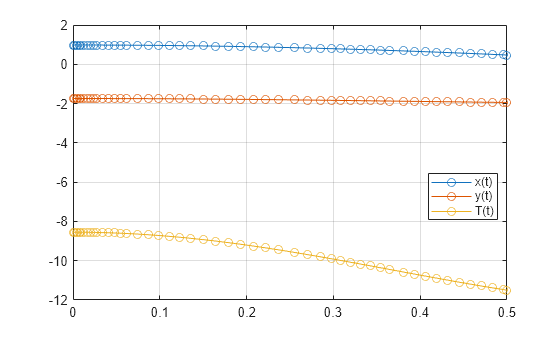
Solve the system integrating over the time span 0 ≤ t ≤ 0.5. Add the grid lines and the legend to the plot. The code uses ode15s. Instead, you can also use ode23t by replacing ode15s with ode23t.

[tSol,ySol] = ode15s(F,[0, 0.5],y0,opt);
plot(tSol,ySol(:,1:origVars),"-o")

for k = 1:origVars
    S{k} = char(DAEvars(k));
end

legend(S,Location="best")
grid on

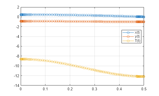
Solve the system for different parameter values by setting the new value and regenerating the function handle and initial conditions.

Set rVal to 2 and regenerate the function handle and initial conditions.

rVal = 2;

F = @(t,Y) f(t,Y,gVal,mVal,rVal);
y0est = [rVal*sin(pi/6); -rVal*cos(pi/6); 0; 0; 0; 0; 0];
implicitDAE = @(t,y,yp) M(t,y)*yp - F(t,y);
[y0,yp0] = decic(implicitDAE,0,y0est,[],yp0est,[],opt);

opt = odeset(opt,InitialSlope=yp0);

Solve the system for the new parameter value.

[tSol,ySol] = ode15s(F,[0, 0.5],y0,opt);
plot(tSol,ySol(:,1:origVars),"-o")

for k = 1:origVars
    S{k} = char(DAEvars(k));
end

legend(S,Location="best")
grid on