Choose an Approach for Solving Equations Using solve Function

Symbolic Math Toolbox™ provides the solve function for solving a mathematical equation or a system of equations. The solve function can return unique solutions, no solutions, or infinitely many solutions that include parameterizations and conditions on the unknowns. However, even when unique solutions exist, the toolbox might not express the solutions in a symbolic form explicitly. For these reasons, you can choose from several approaches to solving equations:

• Find a complete set of solutions, including parameters and conditions on solutions.

• Find numerical solutions with arbitrary precision.

• Find solutions for equations that include the definition of a symbolic function.

• Find other forms of solutions.

This example discusses these approaches. If you want to solve a system of ordinary differential equations, use dsolve instead.

Approaches for Solving Equations

When to Use	Approach	More Information
You want to find a complete set of solutions, including parameters and conditions on solutions. The system of equations to be solved can be consistent or inconsistent.	Use the solve function with ReturnConditions set to true.	Include Parameters and Conditions on Solutions
You want to find numerical solutions with arbitrary precision when solve cannot find a symbolic solution.	Use the vpasolve function instead.	Find Numerical Solutions
You want to solve a system of equations that includes the definition of a symbolic function.	Define the symbolic function outside the system of equations. Solve the system separately and apply necessary substitutions to rewrite the formula of the function.	Define Symbolic Function Outside of Equations
You want to find other forms of solutions.	Use the solve function with name-value arguments: • To return only real solutions, specify Real as true. • To solve inequalities including parameters and conditions on solutions, specify ReturnConditions as true. • To ignore the assumptions on the unknowns, specify IgnoreProperties as true. • To apply mathematical rules that are assumed to be valid, specify IgnoreAnalyticConstraints as true. • To find analytical solutions for polynomials with a degree less than 5, specify MaxDegree as a positive integer less than 5 . • To return one solution out of many possible solutions, specify PrincipalValue as true.	For examples, see: • Solve Polynomial and Return Real Solutions • Solve Inequalities • Ignore Assumptions on Variables • Apply Mathematical Rules • Solve Polynomial Equations of High Degree • Return One Solution

The solve function attempts to find symbolic solutions to your equations. Although specifying ReturnConditions as true is the most comprehensive approach, it is generally the slowest. To increase computational speed, reduce the number of symbolic variables in your equations by substituting given values for some variables before using solve. For further speed improvements, if you are interested only in the solutions without parameterization, consider using the numeric solver vpasolve with a lower precision setting. To use another numeric solver without Symbolic Math Toolbox, you can convert symbolic expressions to MATLAB® functions by using matlabFunction. This conversion allows you to use the resulting function with other solvers in different MATLAB products, such as fsolve (Optimization Toolbox) in Optimization Toolbox™.

Include Parameters and Conditions on Solutions

A system of equations consists of a specific number of equations and unknowns. In mathematics, these systems can be categorized as:

• Overdetermined system — More equations than unknowns

• Underdetermined system — Fewer equations than unknowns

• Exactly determined system — An equal number of equations and unknowns

However, the existence of solutions for these systems is not primarily dependent on the number of equations and unknowns. A system is considered consistent if at least one set of values for the unknowns satisfies all the equations. In this case, the solution might consist of specific values or involve free parameters. In contrast, a system is considered inconsistent if no set of values for the unknowns satisfies all the equations [1].

Consistent and Inconsistent Systems of Equations

A consistent system can involve free parameters in the solutions. To find solutions that include free parameters, specify the ReturnConditions name-value argument as true when using solve.

For example, consider the following system of two equations with three unknowns. This underdetermined system is consistent because a set of solutions for the three unknowns exists. The set of solutions is z = 1 (as seen by subtracting the first equation from the second) and any values of x and y that satisfy x + y = 2.

syms x y z
eq1 = x + y + z == 3;
eq2 = x + y + 2*z == 4;
eqns = [eq1; eq2]

eqns = 
$$\left(\begin{array}{c}x+y+z=3\\ x+y+2\hspace{0.17em}z=4\end{array}\right)$$

Solve this system by using solve. The solver returns one solution from the set of solutions. Here, the solver chooses the solution z = 1, x = 2, and y = 0, which satisfies x + y = 2.

sols = solve(eqns,[x y z])

sols = struct with fields:
    x: 2
    y: 0
    z: 1

To find a complete set of solutions that includes free parameters, specify ReturnConditions as true. Here, the solver returns y = z1 as a free parameter, which can take any complex value.

sols = solve(eqns,[x y z],ReturnConditions=true)

sols = struct with fields:
             x: 2 - z1
             y: z1
             z: 1
    parameters: z1
    conditions: symtrue

Next, consider the following system of equations with two unknowns. This overdetermined system is inconsistent because the last equation contradicts the other two equations (as seen by summing the first two equations).

syms x y
eq1 = x + y == 3;
eq2 = x + 2*y == 7;
eq3 = 2*x + 3*y == 11;
eqns = [eq1; eq2; eq3]

eqns = 
$$\left(\begin{array}{c}x+y=3\\ x+2\hspace{0.17em}y=7\\ 2\hspace{0.17em}x+3\hspace{0.17em}y=11\end{array}\right)$$

The solve function returns an empty solution for this system.

sols = solve(eqns)

sols = struct with fields:
    x: [0×1 sym]
    y: [0×1 sym]

Even if you specify ReturnConditions as true, solve returns an empty solution. These outputs confirm that the system is inconsistent and does not have a solution.

sols = solve(eqns,[x y],ReturnConditions=true)

sols = struct with fields:
             x: [0×1 sym]
             y: [0×1 sym]
    parameters: [1×0 sym]
    conditions: [0×1 sym]

For comparison, solving only two of the three equations yields a solution because no contradiction exists between the two equations.

sols = solve([eq1; eq3])

sols = struct with fields:
    x: -2
    y: 5

Different Parameterizations When Specifying Different Variable Orders

When the solution of a system of equations involves a free parameter, specifying different variable orders to solve for when using solve affects the choice of the unknown to be parameterized.

For example, define a system of equations where the third equation is the result of subtracting the first equation from the second equation.

syms x y z
eq1 = z == 2*x + y;
eq2 = 2*z == 3*x - y;
eq3 = z == x - 2*y;
eqns = [eq1; eq2; eq3];

Solve for x and y. The solver returns the solutions in terms of the other unknown z.

sols = solve(eqns,x,y)

sols = struct with fields:
    x: (3*z)/5
    y: -z/5

Next, solve for y and z. The solver returns the solutions in terms of the other unknown x.

sols = solve(eqns,y,z)

sols = struct with fields:
    y: -x/3
    z: (5*x)/3

Now, if you solve for x, y, and z, then solve returns one solution from the set of solutions that satisfies the system. Here, solve returns x = 0, y = 0, and z = 0.

sols = solve(eqns,x,y,z)

sols = struct with fields:
    x: 0
    y: 0
    z: 0

To find a complete set of solutions that satisfies the system, specify ReturnConditions as true. Here, one unknown has to be parameterized, and the solver selects the last variable you specify in the second input argument to be parameterized. The solver parameterizes the unknown z, which can have any complex value.

sols = solve(eqns,[x y z],ReturnConditions=true)

sols = struct with fields:
             x: (3*z1)/5
             y: -z1/5
             z: z1
    parameters: z1
    conditions: symtrue

For comparison, change the order of the unknowns to solve for in the second input argument. Here, the solver parameterizes the unknown x.

sols = solve(eqns,[y z x],ReturnConditions=true)

sols = struct with fields:
             y: -z1/3
             z: (5*z1)/3
             x: z1
    parameters: z1
    conditions: symtrue

Redundant System of Equations

Consider the following circuit diagram. Define the variables that describe the circuit:

• V1 is the input voltage.

• V2 is the output voltage.

• R1, R2, and R3 are resistors.

• I1 and I2 are currents that flow on specific paths of the circuit.

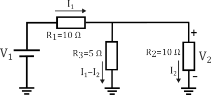
Apply Kirchhoff's voltage and current laws to obtain the system of equations that represents the circuit.

syms V1 V2 I1 I2 R1 R2 R3
eqn1 = -V1 + I1*R1 + (I1-I2)*R3 == 0;
eqn2 = -V1 + I1*R1 + I2*R2 == 0;
eqn3 = -(I1-I2)*R3 + I2*R2 == 0;
eqn4 = V2 == I2*R2;
eqns = [eqn1; eqn2; eqn3; eqn4]

eqns = 
$$\left(\begin{array}{c}{R}_3\hspace{0.17em}\left(I_1-I_2\right)-V_1+I_1\hspace{0.17em}{R}_1=0\\ I_1\hspace{0.17em}{R}_1-V_1+I_2\hspace{0.17em}{R}_2=0\\ I_2\hspace{0.17em}{R}_2-R_3\hspace{0.17em}\left(I_1-I_2\right)=0\\ V_2=I_2\hspace{0.17em}{R}_2\end{array}\right)$$

This system of equations has one equation that is redundant—you can obtain the third equation by subtracting the second equation from the first equation.

For this reason, the system has only three linearly independent equations. You can solve for three unknowns of this system to obtain the result in terms of the other variables that describe the circuit. For example, solve for I1, I2, and V2. The result is in terms of V1, R1, R2, and R3.

sols = solve(eqns,I1,I2,V2)

sols = struct with fields:
    I1: (V1*(R2 + R3))/(R1*R2 + R1*R3 + R2*R3)
    I2: (R3*V1)/(R1*R2 + R1*R3 + R2*R3)
    V2: (R2*R3*V1)/(R1*R2 + R1*R3 + R2*R3)

You can also solve for I1, I2, and R1. The result is in terms of V1, V2, R2, and R3.

sols = solve(eqns,I1,I2,R1)

sols = struct with fields:
    I1: (V2*(R2 + R3))/(R2*R3)
    I2: V2/R2
    R1: (R2*R3*V1 - R2*R3*V2)/(R2*V2 + R3*V2)

If you solve for four unknowns from this system of four equations, where one equation is redundant without specifying ReturnConditions as true, then the solver chooses one solution from the set of solutions that satisfies the system. For example, solving for I1, I2, V1, and V2 results in a solution of 0 for these unknowns.

sols = solve(eqns,I1,I2,V1,V2)

sols = struct with fields:
    I1: 0
    I2: 0
    V1: 0
    V2: 0

For comparison, if you solve for I1, I2, V1, and R2, then the solver chooses a solution where R2 is 1.

sols = solve(eqns,I1,I2,V1,R2)

sols = struct with fields:
    I1: (V2 + R3*V2)/R3
    I2: V2
    V1: (R1*V2 + R3*V2 + R1*R3*V2)/R3
    R2: 1

To find a complete set of solutions that satisfies the system, along with the free parameters and conditions on the solutions, specify ReturnConditions as true. Here, solving for I1, I2, V1, and V2 results in a set of solutions where the solver parameterizes the variable V2.

sols = solve(eqns,I1,I2,V1,V2,ReturnConditions=true)

sols = struct with fields:
            I1: (z*(R2 + R3))/(R2*R3)
            I2: z/R2
            V1: (z*(R1*R2 + R1*R3 + R2*R3))/(R2*R3)
            V2: z
    parameters: z
    conditions: R1 + R3 ~= 0 & R2 ~= 0 & R3 ~= 0 & R1*R2 + R1*R3 + R2*R3 ~= 0

However, if your system of equations is more complicated and involves more unknowns, the solver can be slow, especially if ReturnConditions is set to true. In such cases, if you know the values of the other unknowns, you can substitute these values before using solve to speed up the solver computation.

params.R1 = 10;
params.R2 = 10;
params.R3 = 5;
eqnSubbed = vpa(subs(eqns,params));
sols = solve(eqnSubbed,I1,I2,V1,V2,ReturnConditions=true)

sols = struct with fields:
            I1: 0.3*z
            I2: 0.1*z
            V1: 4.0*z
            V2: z
    parameters: z
    conditions: symtrue

Find Numerical Solutions

If solve cannot find an explicit solution, it can issue a warning and return an empty solution. To overcome this issue, specify the appropriate number of unknowns to solve for to make the system of equations consistent. You can also use vpasolve to find numerical solutions within specific digits of precision.

If solve Cannot Find Explicit Solution

Define a system of equations that involve trigonometric functions.

syms x y z
eqns = [x^2*z*(y-1) == 0; sin(sqrt(3)*x) == z; cos(x) == 1]

eqns = 
$$\left(\begin{array}{c}{x}^2\hspace{0.17em}z\hspace{0.17em}\left(y-1\right)=0\\ \sin \left(\sqrt{3}\hspace{0.17em}x\right)=z\\ \cos \left(x\right)=1\end{array}\right)$$

Solve for only. The solver issues a warning and returns an empty solution.

sols = solve(eqns,x)

Warning: Unable to find explicit solution. For options, see <a href="matlab:web(fullfile(docroot, 'symbolic/troubleshoot-equation-solutions-from-solve-function.html'))">help</a>.

 
sols =
 
Empty sym: 0-by-1
 

Instead, specify x, y, and z as the unknowns to solve for. Here, solve returns two valid solutions.

sols = solve(eqns,[x y z])

sols = struct with fields:
    x: [2×1 sym]
    y: [2×1 sym]
    z: [2×1 sym]

sols.x

ans = 
$$\left(\begin{array}{c}0\\ 0\end{array}\right)$$

sols.y

ans = 
$$\left(\begin{array}{c}1\\ 0\end{array}\right)$$

sols.z

ans = 
$$\left(\begin{array}{c}0\\ 0\end{array}\right)$$

To find the complete set of solutions with parameterization, specify ReturnConditions as true.

sols = solve(eqns,[x y z],ReturnConditions=true)

sols = struct with fields:
             x: [2×1 sym]
             y: [2×1 sym]
             z: [2×1 sym]
    parameters: [k    z1]
    conditions: [2×1 sym]

sols.x

ans = 
$$\left(\begin{array}{c}2\hspace{0.17em}\pi \hspace{0.17em}k\\ 0\end{array}\right)$$

sols.y

ans = 
$$\left(\begin{array}{c}1\\ z_1\end{array}\right)$$

sols.z

ans = 
$$\left(\begin{array}{c}\sin \left(2\hspace{0.17em}\pi \hspace{0.17em}\sqrt{3}\hspace{0.17em}k\right)\\ 0\end{array}\right)$$

sols.conditions

ans = 
$$\left(\begin{array}{c}k\in \mathbb{Z}\\ \mathrm{symtrue}\end{array}\right)$$

If round-off errors are not a significant issue, you can also use vpasolve to find a numerical solution. By default, vpasolve uses 32 digits of precision. For this example, specify 20 digits of precision. Solve for x, y, and z by specifying an initial guess of 0 for all these variables. Here, the numerical solution is identical to one of the symbolic solutions, where x = 0, y = 0, and z = 0.

digits(20)
sols = vpasolve(eqns,[x y z],0)

sols = struct with fields:
    x: 0
    y: 0
    z: 0

Specify the initial guess as 1. Here, vpasolve returns an approximate solution. This solution satisfies the system of equations within the 20 digits of precision (as seen by substituting the solution into the system of equations).

sols = vpasolve(eqns,[x y z],1)

sols = struct with fields:
    x: 0.00000000000000035116234294122756747
    y: 1.0
    z: 0.00000000000000060823101967913224505

vpa(subs(eqns,sols))

ans = 
$$\left(\begin{array}{c}0.0=0.0\\ 0.00000000000000060823101967913224505=0.00000000000000060823101967913224505\\ 1.0=1.0\end{array}\right)$$

Restore the value of digits to 32 for further calculations.

digits(32)

If solve Returns Conditions That Restate the System of Equations

Define the probability density function of the gamma distribution with parameters $\alpha$ and $\beta$.

syms x alpha beta positive
pdf = (beta^alpha)/gamma(alpha)*x^(alpha-1)*exp(-beta*x)

pdf = 
$$\frac{{\beta }^{\alpha }\hspace{0.17em}{x}^{\alpha -1}\hspace{0.17em}{\mathrm{e}}^{-\beta \hspace{0.17em}x}}{\Gamma \text{<a href="matlab:doc symbolic/gamma">gamma</a>}\left(\alpha \right)}$$

Find the mean of this distribution and the cumulative distribution function.

syms xc
integratex = int(x*pdf,x,0,xc);
mean = simplify(limit(integratex,xc,Inf,"left"))

mean = 
$$\frac{\alpha }{\beta }$$

cdf(xc) = int(pdf,x,0,xc)

cdf(xc) = 
$$1-\frac{\Gamma \text{<a href="matlab:doc symbolic/igamma">igamma</a>}(\alpha ,\beta \hspace{0.17em}\mathrm{xc})}{\Gamma \text{<a href="matlab:doc symbolic/gamma">gamma</a>}\left(\alpha \right)}$$

Define two equations that specify the mean of this distribution as 7 and the cumulative distribution function as 0.9 for $0<\mathit{x}\le 10$.

eq1 = mean == 7

eq1 = 
$$\frac{\alpha }{\beta }=7$$

eq2 = cdf(10) == 0.9

eq2 = 
$$1-\frac{\Gamma \text{<a href="matlab:doc symbolic/igamma">igamma</a>}(\alpha ,10\hspace{0.17em}\beta )}{\Gamma \text{<a href="matlab:doc symbolic/gamma">gamma</a>}\left(\alpha \right)}=\frac{9}{10}$$

Solve for the parameters $\alpha$ and $\beta$ using solve. Here, solve issues a warning and returns parameterized solutions.

sols = solve([eq1; eq2],[alpha beta])

Warning: Solutions are parameterized by the symbols: [z, z1], z1. To include parameters and conditions in the solution, specify the 'ReturnConditions' value as 'true'.

Warning: Solutions are only valid under certain conditions. To include parameters and conditions in the solution, specify the 'ReturnConditions' value as 'true'.

sols = struct with fields:
    alpha: z
     beta: z1

Include parameters and conditions on the solutions by specifying ReturnConditions as true. Here, the conditions on the parameterized solution are a restatement of the equations to be solved. In other words, solve cannot find the explicit symbolic solutions.

sols = solve([eq1; eq2],[alpha beta],ReturnConditions=true)

sols = struct with fields:
         alpha: z
          beta: z1
    parameters: [z    z1]
    conditions: 1/10 - igamma(z, 10*z1)/gamma(z) == 0 & z/z1 - 7 == 0 & 0 < z & 0 < z1

Instead, use vpasolve to find a numerical solution for the two equations. To find nonnegative solutions, set the search interval as [0 Inf] for both $\alpha$ and $\beta$.

sols = vpasolve([eq1; eq2],[alpha beta],[0 Inf; 0 Inf])

sols = struct with fields:
    alpha: 9.6391484249254912862751301540044
     beta: 1.3770212035607844694678757362863

If solve Cannot Find Symbolic Solution and Returns Numerical Solution Instead

The solve function attempts to find symbolic solutions to your equations. If solve cannot symbolically solve an equation, it tries to find a numerical solution using vpasolve. By default, the vpasolve function returns the first solution found.

Solve the equation $\sin \left(\mathit{x}\right)={\mathit{x}}^2-1$. solve issues a warning and returns a numeric solution because it cannot find a symbolic solution.

syms x
eqn = sin(x) == x^2 - 1;
sol = solve(eqn,x)

Warning: Unable to solve symbolically. Returning a numeric solution using <a href="matlab:web(fullfile(docroot, 'symbolic/vpasolve.html'))">vpasolve</a>.

sol = $$-0.63673265080528201088799090383828$$

Plot the left and right sides of the equation. The plot shows that the equation also has a positive solution.

fplot([lhs(eqn) rhs(eqn)],[-2 2])

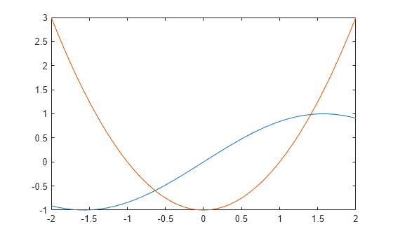
Find the other solution by directly calling the numeric solver vpasolve and specifying the search interval as 0 to 2.

sol2 = vpasolve(eqn,x,[0 2])

sol2 = $$1.4096240040025962492355939705895$$

Define Symbolic Function Outside of Equations

When solving a system of equations that involves symbolic functions, solve might return an empty solution. For example, the following equations define the formula for a function $\mathit{f}\left(\mathit{x}\right)$ and the value of the function at $\mathit{f}\left(1\right)$.

syms f(x) a
eq1 = f(x) == 3*x + a;
eq2 = f(1) == 5;
eqns = [eq1; eq2]

eqns = 
$$\left(\begin{array}{c}f\left(x\right)=a+3\hspace{0.17em}x\\ f\left(1\right)=5\end{array}\right)$$

If you use solve to find the value of $\mathit{a}$, then solve returns an empty solution.

asol = solve(eqns,a)

 
asol =
 
Empty sym: 0-by-1
 

Instead, define the formula for the symbolic function$\mathit{f}\left(\mathit{x}\right)$ outside the system of equations. Then, solve for $\mathit{a}$ by using the evaluated value of $\mathit{f}\left(\mathit{x}\right)$ at 1.

syms f(x) a
f(x) = 3*x + a;
asol = solve(f(1) == 5)

asol = $$2$$

Once you have the solution for $\mathit{a}$, you can substitute it into the original formula.

fsol = subs(f(x),a,asol)

fsol = $$3\hspace{0.17em}x+2$$

References

[1] "Consistent and Inconsistent Equations." In Wikipedia, September 3, 2024. https://en.wikipedia.org/w/index.php?title=Consistent_and_inconsistent_equations&oldid=1243721077.

[2] "Overdetermined System." In Wikipedia, July 22, 2024. https://en.wikipedia.org/w/index.php?title=Overdetermined_system&oldid=1235933306.

[3] "Underdetermined System." In Wikipedia, August 1, 2024. https://en.wikipedia.org/w/index.php?title=Underdetermined_system&oldid=1237892077.