LOWESS, Locally Weighted Scatterplot Smoothing for linear and non-linear data (enhanced)
LOWESS- Locally Weighted Scatterplot Smoothing that does not require the statistical toolbox in matlab.
This regression will work on linear and non-linear relationships between X and Y.
Modifications:
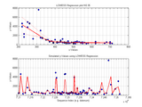
12/19/2008 - added upper and lower LOWESS smooths. These additional smooths show how the distribution of Y varies with X. These smooths are simply LOWESS applied to the positive and negative residuals separately, then added to the original lowess of the data. The same smoothing factor is applied to both the upper and lower limits.
2/21/2009 - added sorting to the function, data no longer need to be sorted. Also added a routine such that if a user also supplies a second dataset, linear interpolations are done one the lowess and used to predict y-values for the supplied x-values.
10/27/2009 - modified the second user provided X-data for obtaining predictions. Matlab function unique sorts by default. It really was not needed in the section of code to perform linear interpolations of the x-data using the y-predicted LOWESS results. If the user does not supply a second x-data set, it will assume to use the supplied x-y data set. Thus there is an output (xy) that maintains the original sequence of the input. Additionally, the user can now include a sequence index as the first column of input data. This can be a datenum or some other ordering index. The output will be sequenced using that index. If a sequence index is provided a second subplot will be created show the predicted Y-values in the order of the included sequence index. I suspect this sequence index most often will be a DateTime (i.e. datenum). Just to the function generic enough, the X-axis labels are not converted to a nice date format, but the user could easily change that with a datetic attribute in the subplot.
6/15/2012 - oddly, when using this routine on data without a time sequence (i.e. a third column), the plotting portions cause an error. Not sure how I would have missed that but...I think I have it fixed.
Using a robust regression like LOWESS allows one the ability to detect a trend in data that may otherwise have too much variance resulting in non-significance p-values.
Yhat (prediction) is computed from a weghted least squares regression whose weights are both a function of distance from X and magnitude from of the residual from the previous regression.
The logic of these functions and subfunctions follow the USGS
Kendall.exe routines. Because matlab is 8-byte precision, there are some very small differences between FORTRAN compiled and matlab. Maybe 64-bit OS's has 16-byte precision in matlab?
Data are expected to be sorted prior to data input for this function. Sorted on first column of datain.
There is a very simple subfucntion to create a plot of the data and regression if the user so choses with a flag in the call to the lowess function. BTW-- the png file looks much better than what the figure looks like on screen.
There are loops in these routines to keep the memory requirements to a minimum, since it is foreseeable that one may have very large datasets to work with.
f = a smoothing factor between 0 and 1. The closer to one, the more smoothing done.
Syntax:
[dataout lowerLimit upperLimit]
= lowess(datain,f,wantplot,imagefile)
datain = n x 2 matrix
dataout = n x 3 matrix
wantplot = scaler (optional)
if ~= 0 then create plot
imagefile = full path and file name where to output the figure to an
png file type at 600 dpi.
e.g. imagefile = 'd:\temp\lowess.png';
where:
datain(:,1) = x
datain(:,2) = y
f = scaler (0 < f < 1)
wantplot = scaler
imagefile = string
datain must be sorted prior to loading into this function on the
x-value. This is not done in the function because the user may want to have the end result be unsorted (e.g. time sort).
dataout(:,1) = x
dataout(:,2) = y
dataout(:,3) = y-prediction (aka yhat)
lowerLimit(:,1) = x with negative residuals
lowerLimit(:,2) = y-prediction of residuals + original y-prediction
upperLimit(:,1) = x with positive residuals
upperLimit(:,2) = y-prediction of residuals + original y-prediction
Requirements: none
Written by
Jeff Burkey
King County Department of Natural Resources and Parks
email: jeff.burkey@kingcounty.gov
12/16/2008
Cite As
Jeff Burkey (2024). LOWESS, Locally Weighted Scatterplot Smoothing for linear and non-linear data (enhanced) (https://www.mathworks.com/matlabcentral/fileexchange/22470-lowess-locally-weighted-scatterplot-smoothing-for-linear-and-non-linear-data-enhanced), MATLAB Central File Exchange. Retrieved .
MATLAB Release Compatibility
Platform Compatibility
Windows macOS LinuxCategories
- AI, Data Science, and Statistics > Statistics and Machine Learning Toolbox > Regression > Linear Regression >
- AI, Data Science, and Statistics > Statistics and Machine Learning Toolbox > Regression > Nonlinear Regression >
Tags
Community Treasure Hunt
Find the treasures in MATLAB Central and discover how the community can help you!
Start Hunting!Discover Live Editor
Create scripts with code, output, and formatted text in a single executable document.
| Version | Published | Release Notes | |
|---|---|---|---|
| 1.4.0.0 | There wasnt really an issue having zero values; rather, when supplying data with no time sequence, the interpolation would error. |
||
| 1.3.0.0 | Updated graphing. Revised input. Includes example data file. Revised output. |
||
| 1.2.0.0 | Added a sorting call. Also added a few lines of code allow the user to supply a second set of x-values to be used for y-predictions using the results of the lowess regression. |
||
| 1.1.0.0 | Added computation of upper and lower smooths of the residuals, also will plot on figure. |
||
| 1.0.0.0 |

