bvp5c
Solve boundary value problem — fifth-order method
Description
sol = bvp5c(odefun,bcfun,solinit)odefun, subject to the boundary conditions
described by bcfun and the initial solution guess
solinit. Use the bvpinit function to create the initial guess solinit, which
also defines the points at which the boundary conditions in bcfun are
enforced.
sol = bvp5c(odefun,bcfun,solinit,options)options, which is an
argument created using the bvpset function. For example, use the
AbsTol and RelTol options to specify absolute and
relative error tolerances, or the FJacobian option to provide the
analytical partial derivatives of odefun.
Examples
Solve a second-order BVP in MATLAB® using functions. For this example, use the second-order equation
.
The equation is defined on the interval subject to the boundary conditions
,
.
To solve this equation in MATLAB, you need to write a function that represents the equation as a system of first-order equations, a function for the boundary conditions, and a function for the initial guess. Then the BVP solver uses these three inputs to solve the equation.
Code Equation
Write a function that codes the equation. Use the substitutions and to rewrite the equation as a system of first-order equations.
,
.
The corresponding function is
function dydx = bvpfcn(x,y)
dydx = zeros(2,1);
dydx = [y(2)
       -y(1)];
end
Note: All functions are included at the end of the example as local functions.
Code Boundary Conditions
Write a function that codes the boundary conditions in the form . In this form the boundary conditions are
,
.
The corresponding function is
function res = bcfcn(ya,yb)
res = [ya(1)
       yb(1)-2];
end
Create Initial Guess
Use the bvpinit function to create an initial guess for the solution of the equation. Since the equation relates to , a reasonable guess is that the solution involves trigonometric functions. Use a mesh of five points in the interval of integration. The first and last values in the mesh are where the solver applies the boundary conditions.
The function for the initial guess accepts as an input and returns a guess for the value of and . The function is
function g = guess(x)
g = [sin(x)
     cos(x)];
end
xmesh = linspace(0,pi/2,5);
solinit = bvpinit(xmesh, @guess);
Solve Equation
Use bvp5c with the derivative function, boundary condition function, and initial guess to solve the problem.
sol = bvp5c(@bvpfcn, @bcfcn, solinit);
Plot Solution
plot(sol.x, sol.y, '-o')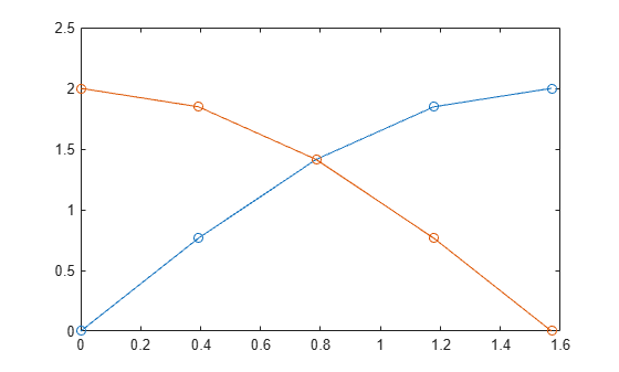
Local Functions
Listed here are the local functions that bvp5c uses to solve the equation.
function dydx = bvpfcn(x,y) % equation to solve
dydx = zeros(2,1);
dydx = [y(2)
       -y(1)];
end
%--------------------------------
function res = bcfcn(ya,yb) % boundary conditions
res = [ya(1)
       yb(1)-2];
end
%--------------------------------
function g = guess(x) % initial guess for y and y'
g = [sin(x)
     cos(x)];
end
%--------------------------------
Solve a BVP at a crude error tolerance with two different solvers and compare the results.
Consider the second-order ODE
.
The equation is defined on the interval subject to the boundary conditions
,
.
To solve this equation in MATLAB®, you need to write a function that represents the equation as a system of first-order equations, write a function for the boundary conditions, set some option values, and create an initial guess. Then the BVP solver uses these four inputs to solve the equation.
Code Equation
With the substitutions and , you can rewrite the ODE as a system of first-order equations
,
.
The corresponding function is
function dydx = bvpfcn(x,y)
dydx = [y(2)
       -2*y(2)/x - y(1)/x^4];
end
Note: All functions are included at the end of the example as local functions.
Code Boundary Conditions
The boundary condition function requires that the boundary conditions are in the form . In this form, the boundary conditions are
,
.
The corresponding function is
function res = bcfcn(ya,yb)
res = [ya(1)
       yb(1)-sin(1)];
end
Set Options
Use bvpset to turn on the display of solver statistics, and specify crude error tolerances to highlight the difference in error control between the solvers. Also, for efficiency, specify the analytical Jacobian
.
The corresponding function that returns the value of the Jacobian is
function dfdy = jac(x,y)
dfdy = [0      1
       -1/x^4 -2/x];
end
opts = bvpset('FJacobian',@jac,'RelTol',0.1,'AbsTol',0.1,'Stats','on');
Create Initial Guess
Use bvpinit to create an initial guess of the solution. Specify a constant function as the initial guess with an initial mesh of 10 points in the interval .
xmesh = linspace(1/(3*pi), 1, 10);
solinit = bvpinit(xmesh, [1; 1]);
Solve Equation
Solve the equation with both bvp4c and bvp5c.
sol4c = bvp4c(@bvpfcn, @bcfcn, solinit, opts);
The solution was obtained on a mesh of 9 points.
The maximum residual is  9.794e-02.
There were 157 calls to the ODE function.
There were 28 calls to the BC function.
sol5c = bvp5c(@bvpfcn, @bcfcn, solinit, opts);
The solution was obtained on a mesh of 11 points.
The maximum error is  6.742e-02.
There were 244 calls to the ODE function.
There were 29 calls to the BC function.
Plot Results
Plot the results of the two calculations for with the analytic solution for comparison. The analytic solution is
,
.
xplot = linspace(1/(3*pi),1,200);
yplot = [sin(1./xplot); -cos(1./xplot)./xplot.^2];

plot(xplot,yplot(1,:),'k',sol4c.x,sol4c.y(1,:),'r*',sol5c.x,sol5c.y(1,:),'bo')
title('Comparison of BVP Solvers with Crude Error Tolerance')
legend('True','BVP4C','BVP5C')
xlabel('x')
ylabel('solution y')
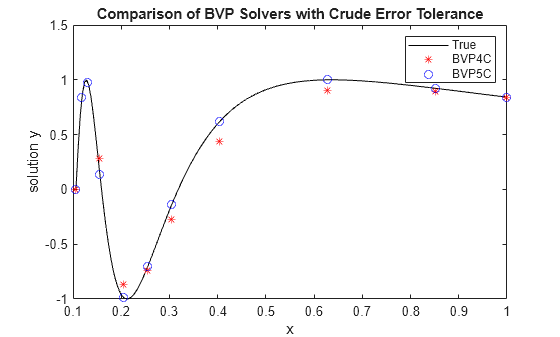
The plot confirms that bvp5c directly controls the true error in the calculation, while bvp4c controls it only indirectly. At more stringent error tolerances, this difference between the solvers is not as apparent.
Local Functions
Listed here are the local functions that the BVP solvers use to solve the problem.
function dydx = bvpfcn(x,y) % equation to solve
dydx = [y(2)
       -2*y(2)/x - y(1)/x^4];
end
%---------------------------------
function res = bcfcn(ya,yb) % boundary conditions
res = [ya(1)
       yb(1)-sin(1)];
end
%---------------------------------
function dfdy = jac(x,y) % analytical jacobian for f
dfdy = [0      1
       -1/x^4 -2/x];
end
%---------------------------------
Input Arguments
Output Arguments
More About
Algorithms
bvp5c is a finite difference code that implements the four-stage
Lobatto IIIa formula [1]. This is a collocation formula and the collocation polynomial
provides a C1-continuous solution that is
fifth-order accurate uniformly in [a,b]. The formula is implemented as an
implicit Runge-Kutta formula. Some of the differences between bvp5c and
bvp4c are:
bvp5csolves the algebraic equations directly.bvp4cuses analytical condensation.bvp4chandles unknown parameters directly.bvp5caugments the system with trivial differential equations for the unknown parameters.
References
[1] Shampine, L.F., and J. Kierzenka. "A BVP Solver that Controls Residual and Error." J. Numer. Anal. Ind. Appl. Math. Vol. 3(1-2), 2008, pp. 27–41.
Extended Capabilities
Version History
Introduced in R2006b