conv2
2-D convolution
Description
C = conv2(A,B)A and B.
If
Ais a matrix andBis a row vector (orAis a row vector andBis a matrix), thenCis the convolution of each row of the matrix with the vector.If
Ais a matrix andBis a column vector (orAis a column vector andBis a matrix), thenCis the convolution of each column of the matrix with the vector.
Examples
In applications such as image processing, it can be useful to compare the input of a convolution directly to the output. The conv2 function allows you to control the size of the output.
Create a 3-by-3 random matrix A and a 4-by-4 random matrix B. Compute the full convolution of A and B, which is a 6-by-6 matrix.
A = rand(3);
B = rand(4);
Cfull = conv2(A,B)
Cfull = 6×6

    0.7861    1.2768    1.4581    1.0007    0.2876    0.0099
    1.0024    1.8458    3.0844    2.5151    1.5196    0.2560
    1.0561    1.9824    3.5790    3.9432    2.9708    0.7587
    1.6790    2.0772    3.0052    3.7511    2.7593    1.5129
    0.9902    1.1000    2.4492    1.6082    1.7976    1.2655
    0.1215    0.1469    1.0409    0.5540    0.6941    0.6499
Compute the central part of the convolution Csame, which is a submatrix of Cfull with the same size as A. Csame is equal to Cfull(3:5,3:5).
Csame = conv2(A,B,"same")Csame = 3×3
3.5790 3.9432 2.9708
3.0052 3.7511 2.7593
2.4492 1.6082 1.7976
The Sobel edge-finding operation uses a 2-D convolution to detect edges in images and other 2-D data.
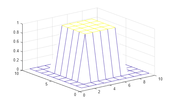
Create and plot a 2-D pedestal with interior height equal to one.
A = zeros(10);
A(3:7,3:7) = ones(5);
mesh(A)
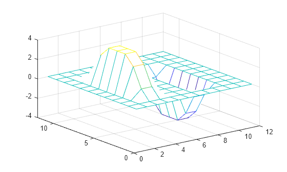
Convolve the rows of A with the vector u, and then convolve the rows of the result with the vector v. The convolution extracts the horizontal edges of the pedestal.
u = [1 0 -1]';
v = [1 2 1];
Ch = conv2(u,v,A);
mesh(Ch)

To extract the vertical edges of the pedestal, reverse the order of convolution with u and v.
Cv = conv2(v,u,A);
mesh(Cv)
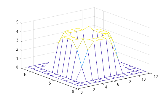
Compute and plot the combined edges of the pedestal.
figure
mesh(sqrt(Ch.^2 + Cv.^2))
Input Arguments
Output Arguments
More About
Extended Capabilities
Version History
Introduced before R2006a