eigs
Subset of eigenvalues and eigenvectors
Syntax
Description
d = eigs(A,k,sigma,Name,Value)eigs(A,k,sigma,'Tolerance',1e-3) adjusts the
convergence tolerance for the algorithm.
Examples
The matrix A = delsq(numgrid('C',15)) is a symmetric positive definite matrix with eigenvalues reasonably well-distributed in the interval (0 8). Compute the six largest magnitude eigenvalues.
A = delsq(numgrid('C',15));
d = eigs(A)
d = 6×1
7.8666
7.7324
7.6531
7.5213
7.4480
7.3517
Specify a second input to compute a specific number of the largest eigenvalues.
d = eigs(A,3)
d = 3×1

    7.8666
    7.7324
    7.6531
The matrix A = delsq(numgrid('C',15)) is a symmetric positive definite matrix with eigenvalues reasonably well-distributed in the interval (0 8). Compute the five smallest eigenvalues.
A = delsq(numgrid('C',15));
d = eigs(A,5,'smallestabs')
d = 5×1

    0.1334
    0.2676
    0.3469
    0.4787
    0.5520
Create a 1500-by-1500 random sparse matrix with a 25% approximate density of nonzero elements.
n = 1500;
A = sprand(n,n,0.25);
Find the LU factorization of the matrix, returning a permutation vector p that satisfies A(p,:) = L*U.
[L,U,p] = lu(A,'vector');Create a function handle Afun that accepts a vector input x and uses the results of the LU decomposition to, in effect, return A\x.
Afun = @(x) U\(L\(x(p)));
Calculate the six smallest magnitude eigenvalues using eigs with the function handle Afun. The second input is the size of A.
d = eigs(Afun,1500,6,'smallestabs')d = 6×1 complex
0.1423 + 0.0000i
0.4859 + 0.0000i
-0.3323 - 0.3881i
-0.3323 + 0.3881i
0.1019 - 0.5381i
0.1019 + 0.5381i
west0479 is a real-valued 479-by-479 sparse matrix with both real and complex pairs of conjugate eigenvalues.
Load the west0479 matrix, then compute and plot all of the eigenvalues using eig. Since the eigenvalues are complex, plot automatically uses the real parts as the x-coordinates and the imaginary parts as the y-coordinates.
load west0479
A = west0479;
d = eig(full(A));
plot(d,'+')
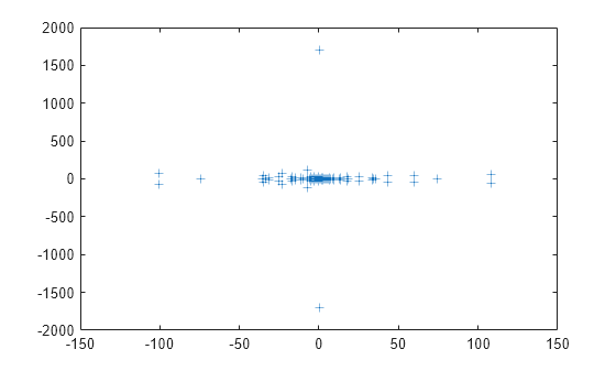
The eigenvalues are clustered along the real line (x-axis), particularly near the origin.
eigs has several options for sigma that can pick out the largest or smallest eigenvalues of varying types. Compute and plot some eigenvalues for each of the available options for sigma.
figure
plot(d, '+')
hold on
la = eigs(A,6,'largestabs');
plot(la,'ro')
sa = eigs(A,6,'smallestabs');
plot(sa,'go')
hold off
legend('All eigenvalues','Largest magnitude','Smallest magnitude')
xlabel('Real axis')
ylabel('Imaginary axis')
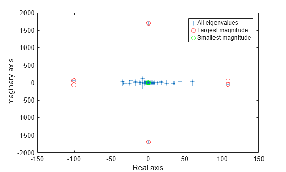
figure
plot(d, '+')
hold on
ber = eigs(A,4,'bothendsreal');
plot(ber,'r^')
bei = eigs(A,4,'bothendsimag');
plot(bei,'g^')
hold off
legend('All eigenvalues','Both ends real','Both ends imaginary')
xlabel('Real axis')
ylabel('Imaginary axis')
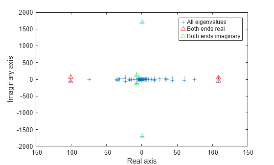
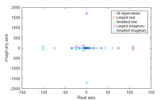
figure
plot(d, '+')
hold on
lr = eigs(A,3,'largestreal');
plot(lr,'ro')
sr = eigs(A,3,'smallestreal');
plot(sr,'go')
li = eigs(A,3,'largestimag','SubspaceDimension',45);
plot(li,'m^')
si = eigs(A,3,'smallestimag','SubspaceDimension',45);
plot(si,'c^')
hold off
legend('All eigenvalues','Largest real','Smallest real','Largest imaginary','Smallest imaginary')
xlabel('Real axis')
ylabel('Imaginary axis')
Create a symmetric positive definite sparse matrix.
A = delsq(numgrid('C', 150));Compute the six smallest real eigenvalues using 'smallestreal', which employs a Krylov method using A.
tic
d = eigs(A, 6, 'smallestreal')
d = 6×1
0.0013
0.0025
0.0033
0.0045
0.0052
0.0063
toc
Elapsed time is 0.747488 seconds.
Compute the same eigenvalues using 'smallestabs', which employs a Krylov method using the inverse of A.
tic
dsm = eigs(A, 6, 'smallestabs')
dsm = 6×1
0.0013
0.0025
0.0033
0.0045
0.0052
0.0063
toc
Elapsed time is 0.185806 seconds.
The eigenvalues are clustered near zero. The 'smallestreal' computation struggles to converge using A since the gap between the eigenvalues is so small. Conversely, the 'smallestabs' option uses the inverse of A, and therefore the inverse of the eigenvalues of A, which have a much larger gap and are therefore easier to compute. This improved performance comes at the cost of factorizing A, which is not necessary with 'smallestreal'.
Compute eigenvalues near a numeric sigma value that is nearly equal to an eigenvalue.
The matrix A = delsq(numgrid('C',30)) is a symmetric positive definite matrix of size 632 with eigenvalues reasonably well-distributed in the interval (0 8), but with 18 eigenvalues repeated at 4.0. To calculate some eigenvalues near 4.0, it is reasonable to try the function call eigs(A,20,4.0). However, this call computes the largest eigenvalues of the inverse of A - 4.0*I, where I is an identity matrix. Because 4.0 is an eigenvalue of A, this matrix is singular and therefore does not have an inverse. eigs fails and produces an error message. The numeric value of sigma cannot be exactly equal to an eigenvalue. Instead, you must use a value of sigma that is near but not equal to 4.0 to find those eigenvalues.
Compute all of the eigenvalues using eig, and the 20 eigenvalues closest to 4 - 1e-6 using eigs to compare results. Plot the eigenvalues calculated with each method.
A = delsq(numgrid('C',30));
sigma = 4 - 1e-6;
d = eig(A);
D = sort(eigs(A,20,sigma));plot(d(307:326),'ks') hold on plot(D,'k+') hold off legend('eig(A)','eigs(A,20,sigma)') title('18 Repeated Eigenvalues of A')

Create sparse random matrices A and B that both have low densities of nonzero elements.
B = sprandn(1e3,1e3,0.001) + speye(1e3);
B = B'*B;
A = sprandn(1e3,1e3,0.005);
A = A+A';
Find the Cholesky decomposition of matrix B, using three outputs to return the permutation vector s and test value p.
[R,p,s] = chol(B,'vector');
p
p = 0
Since p is zero, B is a symmetric positive definite matrix that satisfies B(s,s) = R'*R.
Calculate the six largest magnitude eigenvalues and eigenvectors of the generalized eigenvalue problem involving A and R. Since R is the Cholesky factor of B, specify 'IsCholesky' as true. Furthermore, since B(s,s) = R'*R and thus R = chol(B(s,s)), use the permutation vector s as the value of 'CholeskyPermutation'.
[V,D,flag] = eigs(A,R,6,'largestabs','IsCholesky',true,'CholeskyPermutation',s);
flag
flag =
0
Since flag is zero, all of the eigenvalues converged.
Input Arguments
Name-Value Arguments
Output Arguments
Tips
eigsgenerates the default starting vector using a private random number stream to ensure reproducibility across runs. Setting the random number generator state usingrngbefore callingeigsdoes not affect the output.Using
eigsis not the most efficient way to find a few eigenvalues of small, dense matrices. For such problems, it might be quicker to useeig(full(A)). For example, finding three eigenvalues in a 500-by-500 matrix is a relatively small problem that is easily handled witheig.If
eigsfails to converge for a given matrix, increase the number of Lanczos basis vectors by increasing the value of'SubspaceDimension'. As secondary options, adjusting the maximum number of iterations,'MaxIterations', and the convergence tolerance,'Tolerance', also can help with convergence behavior.
References
[1] Stewart, G.W. "A Krylov-Schur Algorithm for Large Eigenproblems." SIAM Journal of Matrix Analysis and Applications. Vol. 23, Issue 3, 2001, pp. 601–614.
[2] Lehoucq, R.B., D.C. Sorenson, and C. Yang. ARPACK Users' Guide. Philadelphia, PA: SIAM, 1998.