spline
Cubic spline data interpolation
Description
Examples
Use spline to interpolate a sine curve over unevenly-spaced sample points.
x = [0 1 2.5 3.6 5 7 8.1 10];
y = sin(x);
xx = 0:.25:10;
yy = spline(x,y,xx);
plot(x,y,'o',xx,yy)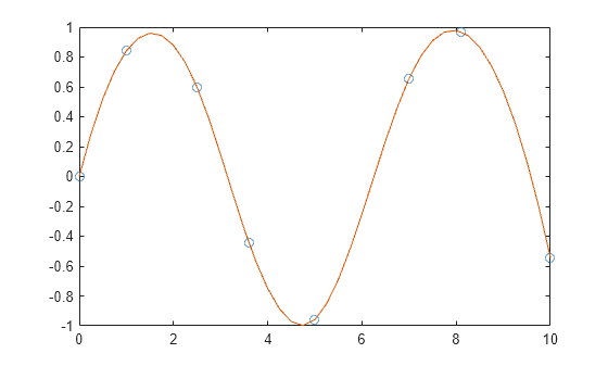
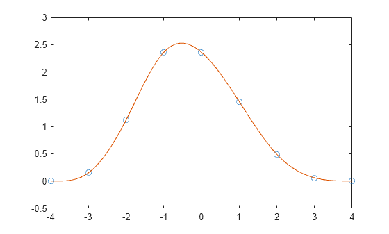
Use clamped or complete spline interpolation when endpoint slopes are known. To do this, you can specify the values vector with two extra elements, one at the beginning and one at the end, to define the endpoint slopes.
Create a vector of data and another vector with the -coordinates of the data.
x = -4:4;
y = [0 .15 1.12 2.36 2.36 1.46 .49 .06 0];
Interpolate the data using spline and plot the results. Specify the second input with two extra values [0 y 0] to signify that the endpoint slopes are both zero. Use ppval to evaluate the spline fit over 101 points in the interpolation interval.
cs = spline(x,[0 y 0]);
xx = linspace(-4,4,101);
plot(x,y,'o',xx,ppval(cs,xx),'-');
Extrapolate a data set to predict population growth.
Create two vectors to represent the census years from 1900 to 1990 (t) and the corresponding United States population in millions of people (p).
t = 1900:10:1990;
p = [ 75.995  91.972  105.711  123.203  131.669 ...
     150.697 179.323  203.212  226.505  249.633 ];
Extrapolate and predict the population in the year 2000 using a cubic spline.
spline(t,p,2000)
ans =
270.6060
Generate the plot of a circle, with the five data points y(:,2),...,y(:,6) marked with o's. The matrix y contains two more columns than does x. Therefore, spline uses y(:,1) and y(:,end) as the endslopes. The circle starts and ends at the point (1,0), so that point is plotted twice.
x = pi*[0:.5:2];
y = [0  1  0 -1  0  1  0;
     1  0  1  0 -1  0  1];
pp = spline(x,y);
yy = ppval(pp, linspace(0,2*pi,101));
plot(yy(1,:),yy(2,:),'-b',y(1,2:5),y(2,2:5),'or')
axis equal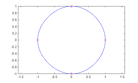
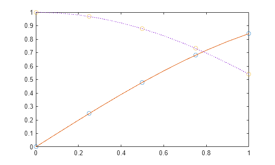
Use spline to sample a function over a finer mesh.
Generate sine and cosine curves for a few values between 0 and 1. Use spline interpolation to sample the functions over a finer mesh.
x = 0:.25:1;
Y = [sin(x); cos(x)];
xx = 0:.1:1;
YY = spline(x,Y,xx);
plot(x,Y(1,:),'o',xx,YY(1,:),'-')
hold on
plot(x,Y(2,:),'o',xx,YY(2,:),':')
hold off
Compare the interpolation results produced by spline, pchip, and makima for two different data sets. These functions all perform different forms of piecewise cubic Hermite interpolation. Each function differs in how it computes the slopes of the interpolant, leading to different behaviors when the underlying data has flat areas or undulations.
Compare the interpolation results on sample data that connects flat regions. Create vectors of x values, function values at those points y, and query points xq. Compute interpolations at the query points using spline, pchip, and makima. Plot the interpolated function values at the query points for comparison.
x = -3:3;
y = [-1 -1 -1 0 1 1 1];
xq1 = -3:.01:3;
p = pchip(x,y,xq1);
s = spline(x,y,xq1);
m = makima(x,y,xq1);
plot(x,y,'o',xq1,p,'-',xq1,s,'-.',xq1,m,'--')
legend('Sample Points','pchip','spline','makima','Location','SouthEast')
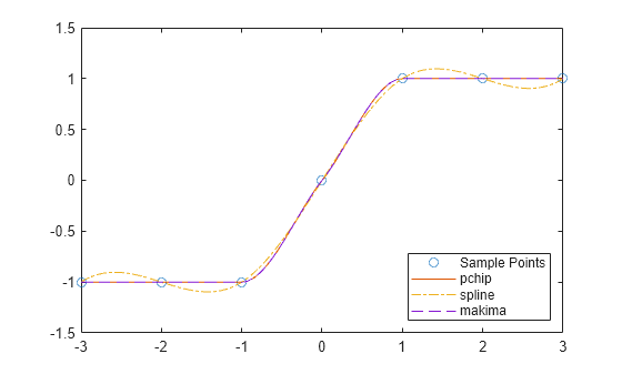
In this case, pchip and makima have similar behavior in that they avoid overshoots and can accurately connect the flat regions.
Perform a second comparison using an oscillatory sample function.
x = 0:15;
y = besselj(1,x);
xq2 = 0:0.01:15;
p = pchip(x,y,xq2);
s = spline(x,y,xq2);
m = makima(x,y,xq2);
plot(x,y,'o',xq2,p,'-',xq2,s,'-.',xq2,m,'--')
legend('Sample Points','pchip','spline','makima')
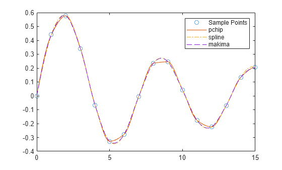
When the underlying function is oscillatory, spline and makima capture the movement between points better than pchip, which is aggressively flattened near local extrema.
Input Arguments
Output Arguments
Tips
You also can perform spline interpolation using the
interp1function with the commandinterp1(x,y,xq,'spline'). Whilesplineperforms interpolation on rows of an input matrix,interp1performs interpolation on columns of an input matrix.
Algorithms
A tridiagonal linear system (possibly with several right-hand
sides) is solved for the information needed to describe the coefficients
of the various cubic polynomials that make up the interpolating spline. spline uses
the functions ppval, mkpp,
and unmkpp. These routines form a small suite
of functions for working with piecewise polynomials. For access to
more advanced features, see interp1 or
the Curve Fitting Toolbox™ spline functions.
References
[1] de Boor, Carl. A Practical Guide to Splines. Springer-Verlag, New York: 1978.
Extended Capabilities
Version History
Introduced before R2006a