AWGN Channel
Add white Gaussian noise to input signal
Libraries:
Communications Toolbox /
Channels
Description
The AWGN Channel block adds white Gaussian noise to the input signal. It inherits the sample time from the input signal.
Examples
This example shows how to adjust the Eb/N0 setting for the AWGN channel to account for the coding rate when your simulation uses coding.
The slex_hamming_check.slx model performs forward error correction (FEC) coding on a BPSK-modulated signal that gets filtered through an AWGN channel. The model uses BPSK Modulator Baseband, AWGN Channel, and BPSK Demodulator Baseband discrete blocks to simulate a binary symmetric channel. To account for difference between the coded and uncoded Eb/N0, the AWGN channel block computes the coded Eb/N0 as Eb/N0 + 10log10(K/N) dB, where K/N is the code rate and Eb/N0 is the uncoded Eb/N0. The Hamming Encoder block has an input bit period of 1 second and the output bit period decreases, by a factor of the K/N code rate, to 4/7 seconds. Due to the coding rate, the Binary Symmetric Channel has a bit period of 4/7 seconds.
The model initializes variables used to configure block parameters by using the PreLoadFcn callback function. For more information, see Model Callbacks (Simulink).
model = 'slex_hamming_check';
open_system(model);

The AWGN channel block must also configure the Number of bits per symbol and Input signal power, referenced to 1 ohm (watts) parameter settings based on the modulated signal. This example uses BPSK modulation, so the AWGN Channel block has the number of bits per symbol set to 1. The model includes a Power Meter block that measures the signal power at the AWGN input to confirm the setting required for the input signal power of the AWGN Channel block.
To compare simulation with theory, produce error rate results and a plot. The theoretical channel error probability for the coded signal is Q(sqrt(2*Ebc/N0)), where Q() is the standard Q function and Ebc/N0 is the coded Eb/N0 in linear units (not in dB). Compute the theoretical BER upper limit bound of a linear, rate 4/7 block code with a minimum distance of 3, and hard decision decoding for a BPSK-modulated signal in AWGN over a range of Eb/N0 values by using the bercodingslex_hamming_check model over the same range of Eb/N0 values.
EbNoVec = 0:2:10;
theorBER = bercoding(EbNoVec,'block','hard',7,4,3);

berVecBSC  = zeros(length(EbNoVec),3);
for n   = 1:length(EbNoVec)
    EbNo = EbNoVec(n);
    sim(model);
    berVecBSC(n,:) = berBSC(end,1);
end
Plot the results by using the semilogy function to show the nearly identical results. The model has the Error Rate Calculation block configured to run each Eb/N0 point until 200 errors occur or the block receives 10^6 bits.
semilogy( ...
    EbNoVec,berVecBSC(:,1),'d', ...
    EbNoVec,theorBER,'-');
legend('BSC BER','Theoretical BER', ...
    Location="southwest");
xlabel("Eb/N0 (dB)");
ylabel("Error Probability");
title("Bit Error Probability");
grid on;

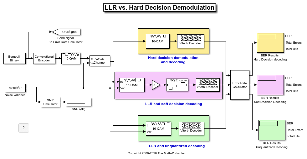
This model shows the improvement in BER performance when using log-likelihood ratio (LLR) instead of hard decision demodulation in a convolutionally coded communication link.
For a MATLAB® version of this example, see Log-Likelihood Ratio (LLR) Demodulation.
System Setup
This example model simulates a convolutionally coded communication system having one transmitter, an AWGN channel and three receivers. The convolutional encoder has a code rate of 1/2. The system employs a 16-QAM modulation. The modulated signal passes through an additive white Gaussian noise channel. The top receiver performs hard decision demodulation in conjunction with a Viterbi decoder that is set up to perform hard decision decoding. The second receiver has the demodulator configured to compute log-likelihood ratios (LLRs) that are then quantized using a 3-bit quantizer. It is well known that the quantization levels are dependent on noise variance for optimum performance [2]. The exact boundaries of the quantizer are empirically determined here. A Viterbi decoder that is set up for soft decision decoding processes these quantized values. The LLR values computed by the demodulator are multiplied by -1 to map them to the right quantizer index for use with Viterbi Decoder. To compute the LLR, the demodulator must be given the variance of noise as seen at its input. The third receiver includes a demodulator that computes LLRs which are processed by a Viterbi decoder that is set up in unquantized mode. The BER performance of each receiver is computed and displayed.
modelName = 'commLLRvsHD';
open_system(modelName);
System Simulation and Visualization
Simulate this system over a range of information bit Eb/No values. Adjust these Eb/No values for coded bits and multi-bit symbols to get noise variance values required for the AWGN block and Rectangular QAM Baseband Demodulator block. Collect BER results for each Eb/No value and visualize the results.
EbNo     = 2:0.5:8; % information rate Eb/No in dB
codeRate = 1/2;     % code rate of convolutional encoder
nBits    = 4;       % number of bits in a 16-QAM symbol
Pavg     = 10;      % average signal power of a 16-QAM modulated signal
snr      = EbNo - 10*log10(1/codeRate) + 10*log10(nBits); % SNR in dB
noiseVarVector = Pavg ./ (10.^(snr./10)); % noise variance

% Initialize variables for storing the BER results
ber_HD  = zeros(1,length(EbNo));
ber_SD  = zeros(1,length(EbNo));
ber_LLR = zeros(1, length(EbNo));

% Loop over all noiseVarVector values
for idx=1:length(noiseVarVector)
    noiseVar = noiseVarVector(idx); %#ok<NASGU>
    sim(modelName);
    % Collect BER results
    ber_HD(idx)  = BER_HD(1);
    ber_SD(idx)  = BER_SD(1);
    ber_LLR(idx) = BER_LLR(1);
end

% Perform curve fitting and plot the results
fitBER_HD  = real(berfit(EbNo,ber_HD));
fitBER_SD  = real(berfit(EbNo,ber_SD));
fitBER_LLR = real(berfit(EbNo,ber_LLR));
semilogy(EbNo,ber_HD,'r*', ...
    EbNo,ber_SD,'g*', ...
    EbNo,ber_LLR,'b*', ...
    EbNo,fitBER_HD,'r', ...
    EbNo,fitBER_SD,'g', ...
    EbNo,fitBER_LLR,'b');
legend('Hard Decision Decoding', ...
    'Soft Decision Decoding','Unquantized Decoding');
xlabel('Eb/No (dB)');
ylabel('BER');
title('LLR vs. Hard Decision Demodulation with Viterbi Decoding');
grid on;

To experiment with this system further, try different modulation types. This system uses a binary mapped modulation scheme for faster error collection but it is well known that Gray mapped signal constellation provides better BER performance. Experiment with various constellation ordering options in the modulator and demodulator blocks. Configure the demodulator block to compute approximate LLR to see the difference in the BER performance compared to hard decision demodulation and LLR. Try out a different range of Eb/No values. Finally, investigate different quantizer boundaries for your modulation scheme and Eb/No values.
Using Dataflow in Simulink
You can configure this example to use data-driven execution by setting the Domain parameter to dataflow for Dataflow Subsystem. With dataflow, blocks inside the domain, execute based on the availability of data as rather than the sample timing in Simulink®. Simulink automatically partitions the system into concurrent threads. This autopartitioning accelerates simulation and increases data throughput. To learn more about dataflow and how to run this example using multiple threads, see Multicore Simulation of Comparing Demodulation Types.
% Cleanup
close_system(modelName,0);
clear modelName EbNo codeRate nBits Pavg snr noiseVarVector ...
    ber_HD ber_SD ber_LLR idx noiseVar fitBER_HD fitBER_SD fitBER_LLR;
Selected Bibliography
[1] J. L. Massey, "Coding and Modulation in Digital Communications", Proc. Int. Zurich Seminar on Digital Communications, 1974
[2] J. A. Heller, I. M. Jacobs, "Viterbi Decoding for Satellite and Space Communication", IEEE® Trans. Comm. Tech. vol COM-19, October 1971
This example uses the doc_gray_code to compute bit error rates (BER) and symbol error rates (SER) for M-PSK modulation. The theoretical error rate performance of M-PSK modulation in AWGN is compared to the error rate performance for Gray-coded symbol mapping and to the error rate performance of binary-coded symbol mapping.
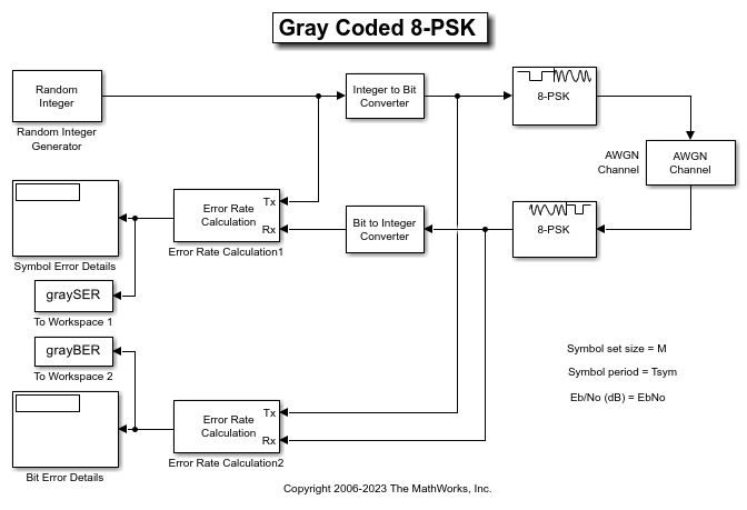
The Random Integer Generator block serves as the source, producing a sequence of integers. The Integer to Bit Converter block converts each integer into a corresponding binary representation. The M-PSK Modulator Baseband block in the doc_gray_code model:
Accepts binary-valued inputs that represent integers in the range [0, (M - 1], where M is the modulation order.
Maps binary representations to constellation points using a Gray-coded ordering.
Produces unit-magnitude complex phasor outputs, with evenly spaced phases in the range [0, (2
 (M - 1) / M)].
The AWGN Channel block adds white Gaussian noise to the modulated data. The M-PSK Demodulator Baseband block demodulates the noisy data. The Bit to Integer Converter block converts each binary representation to a corresponding integer. Then two separate Error Rate Calculation blocks calculate the error rates of the demodulated data. The block labeled SER Calculation compares the integer data to compute the symbol error rate statistics and the block labeled BER Calculation compares the bits data to compute the bit error rate statistics. The output of the Error Rate Calculation block is a three-element vector containing the calculated error rate, the number of errors observed, and the amount of data processed.
To reduce simulation run time and ensure that the statistics of the errors remain stable as the Eb/N0 ratio increases, the model is configured to run until 100 errors occur or until 1e8 bits have been transmitted.
The model initializes variables used to configure block parameters by using the PreLoadFcn callback function. For more information, see Model Callbacks (Simulink).
Produce Error Rate Curves
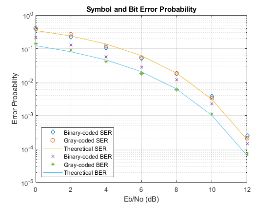
Compute the theoretical BER for nondifferential 8-PSK in AWGN over a range of Eb/N0 values by using the berawgndoc_gray_code model with Gray-coded symbol mapping over the same range of Eb/N0 values.
Compare Gray coding with binary coding, by modifying the M-PSK Modulator Baseband and M-PSK Demodulator Baseband blocks to set the Constellation ordering parameter to Binary instead of Gray. Simulate the doc_gray_code model with binary-coded symbol mapping over the same range of Eb/N0 values.
Plot the results by using the semilogy function. The Gray-coded system achieves better error rate performance than the binary-coded system. Further, the Gray-coded error rate aligns with the theoretical error rate statistics.
The Raised Cosine Transmit Filter and Raised Cosine Receive Filter blocks are designed for raised cosine (RC) filtering. Each block can apply a square-root raised cosine (RRC) filter or a raised cosine filter to a signal. You can vary the roll-off factor and span of the filter.
The Raised Cosine Transmit Filter and Raised Cosine Receive Filter blocks are tailored for use at the transmitter and receiver, respectively. The transmit filter upsamples (interpolates) the output signal. The receive filter expects its input signal to be upsampled and downsamples (decimates) the output signal, based on the configured settings of the block.
The raised cosine transmit and receive filter blocks each introduce a propagation delay, as described in Group Delay.
The doc_rrcfiltercompare.slx model shows how to split the filtering equally between the transmitter and the receiver by using a pair of square root raised cosine filters. The use of a matched pair of square root raised cosine filters is equivalent to a single normal raised cosine filter. The filters share the same span and use the same number samples per symbol but the two filter blocks on the upper path have a square root shape and the single filter block on the lower path has the normal shape.

Run the model and observe the eye and constellation diagrams. The performance is nearly identical for the two methods. Note that the limited impulse response of practical square root raised cosine filters causes a slight difference between the response of two cascaded square root raised cosine filters and the response of one raised cosine filter.


Simulate the model, slex_hamming_check, in parallel by sweeping over  values. An array of
 Simulink.SimulationInput (Simulink) objects is input to parsim (Simulink) to perform the sweep in parallel.
Configure Simulation
model = 'slex_hamming_check.slx';
% Specify sweep values.
EbNoSweep = 0:2:8;
% Create an array of SimulationInput objects.
for i = length(EbNoSweep):-1:1
    in(i) = Simulink.SimulationInput(model);
    in(i) = in(i).setVariable('EbNo',EbNoSweep(i));
end
Run Sweep Simulation
Simulate the model in parallel.
out = parsim(in,'ShowSimulationManager','on')
[20-Apr-2026 06:51:23] Checking for availability of parallel pool...
[20-Apr-2026 06:51:26] Running simulations...
[20-Apr-2026 06:51:58] Completed 1 of 5 simulation runs
[20-Apr-2026 06:52:00] Completed 2 of 5 simulation runs
[20-Apr-2026 06:52:01] Completed 3 of 5 simulation runs
[20-Apr-2026 06:52:02] Completed 4 of 5 simulation runs
[20-Apr-2026 06:52:12] Completed 5 of 5 simulation runs

out =

1x5 Simulink.SimulationOutput array
Low BER Runs
For higher values, simulations require many bits to accumulate enough bit errors for meaningful results. To parallelize the runs for a single , you must ensure relevant blocks have different initial seed values for random number streams in each run.
seedSweep = randi(1e4,5,1);
EbNo = 20;
for i = length(seedSweep):-1:1
    in(i) = Simulink.SimulationInput(model);
    in(i) = in(i).setVariable('seed',seedSweep(i));
end
Run Seed Sweep Simulation
Simulate the model in parallel.
out = parsim(in,'ShowSimulationManager','on')
[20-Apr-2026 06:52:14] Checking for availability of parallel pool...
[20-Apr-2026 06:52:14] Running simulations...
[20-Apr-2026 06:52:24] Completed 1 of 5 simulation runs
[20-Apr-2026 06:52:33] Completed 2 of 5 simulation runs
[20-Apr-2026 06:52:42] Completed 3 of 5 simulation runs
[20-Apr-2026 06:52:52] Completed 4 of 5 simulation runs
[20-Apr-2026 06:53:02] Completed 5 of 5 simulation runs

out =

1x5 Simulink.SimulationOutput array
Limitations
To use this block in a For Each Subsystem (Simulink) you must set
Random number sourcetoGlobal Streamand the model toNormalorAcceleratorsimulation mode. This ensures that each run will generate independent noise samples.
Ports
Input
Output
Parameters
Block Characteristics
Data Types |
|
Multidimensional Signals |
|
Variable-Size Signals |
|
Tips
When running Monte Carlo simulations using generated code or in rapid acceleration more, it is important to ensure that each run uses a different stream of random numbers. To do this:
Set Random number source to
mt19937ar with seed.Make sure that all relevant blocks have different Initial seed values, especially when running simulations in parallel using the
parsim(Simulink) function. For an example, see Simulate Channel Model in Parallel with parsim.
If you do not set different seeds, different workers may generate identical random numbers, which can lead to misleading results. This issue is particularly relevant for models that:
Use rapid accelerator mode.
Contain blocks configured with Simulate using set to
Code generationand Random number source set toGlobal stream.
For more information, see Choosing a Simulation Mode (Simulink).
Algorithms
References
[1] Proakis, John G. Digital Communications. 4th Ed. McGraw-Hill, 2001.