Main Content

bodeoptions

Create list of Bode plot options

Description

Use the bodeoptions command to create a BodeOptions object to customize Bode plot appearance. You can also use the command to override the plot preference settings in the MATLAB® session in which you create the Bode plots.

Creation

Description

example

plotoptions = bodeoptions returns a default set of plot options for use with the bodeplot command. You can use these options to customize the Bode plot appearance using the command line. This syntax is useful when you want to write a script to generate plots that look the same regardless of the preference settings of the MATLAB session in which you run the script.

example

plotoptions = bodeoptions('cstprefs') initializes the plot options with the options you selected in the Control System Toolbox™ and System Identification Toolbox™ Preferences Editor. For more information about the editor, see Toolbox Preferences Editor. This syntax is useful when you want to change a few plot options but otherwise use your default preferences. A script that uses this syntax may generate results that look different when run in a session with different preferences.

Properties

expand all

Frequency units, specified as one of the following values:

  • 'Hz'

  • 'rad/s'

  • 'rpm'

  • 'kHz'

  • 'MHz'

  • 'GHz'

  • 'rad/nanosecond'

  • 'rad/microsecond'

  • 'rad/millisecond'

  • 'rad/minute'

  • 'rad/hour'

  • 'rad/day'

  • 'rad/week'

  • 'rad/month'

  • 'rad/year'

  • 'cycles/nanosecond'

  • 'cycles/microsecond'

  • 'cycles/millisecond'

  • 'cycles/hour'

  • 'cycles/day'

  • 'cycles/week'

  • 'cycles/month'

  • 'cycles/year'

Frequency scale, specified as either 'log' or 'linear'.

Magnitude units, specified as either 'dB' or absolute value 'abs'.

Magnitude scale, specified as either 'log' or 'linear'.

Toggle magnitude plot visibility, specified as either 'on' or 'off'.

Lower magnitude limit mode, specified as either 'auto' or 'manual'.

Lower magnitude limit value, specified as a scalar.

Phase units, specified as either 'deg' or 'rad' to change to degrees or radians, respectively.

Toggle phase plot visibility, specified as either 'on' or 'off'.

Enable phase wrapping, specified as either 'on' or 'off'. When you set PhaseWrapping to 'on', the plot wraps accumulated phase at the value specified by the PhaseWrappingBranch property.

Phase wrapping value at which the plot wraps accumulated phase when PhaseWrapping is set to 'on'. By default, phase wraps into the interval [-180°,180°].

Enable phase matching, specified as either 'on' or 'off'. Turning PhaseMatching 'on' matches the phase to the value specified in PhaseMatchingValue at the frequency specified in PhaseMatchingFreq.

Phase matching frequency, specified as a scalar.

Phase matching response value, specified as a scalar.

Number of standard deviations to use to plot the confidence region, specified as a scalar. This is applicable to identified models only.

Grouping of input-output (I/O) pairs, specified as one of the following:

  • 'none' — No input-output grouping.

  • 'inputs' — Group only the inputs.

  • 'outputs' — Group only the outputs.

  • 'all' — Group all the I/O pairs.

Input label style, specified as a structure with the following fields:

  • FontSize — Font size, specified as a scalar value greater than zero in point units. The default font size depends on the specific operating system and locale. One point equals 1/72 inch.

  • FontWeight — Character thickness, specified as 'Normal' or 'bold'. MATLAB uses the FontWeight property to select a font from those available on your system. Not all fonts have a bold weight. Therefore, specifying a bold font weight can still result in the normal font weight.

  • FontAngle — Character slant, specified as 'Normal' or 'italic'. Not all fonts have both font styles. Therefore, the italic font might look the same as the normal font.

  • Color — Text color, specified as an RGB triplet. The default color is dark grey with the RGB triplet [0.4,0.4,0.4].

  • Interpreter — Text interpreter, specified as one of these values:

    • 'tex' — Interpret characters using a subset of TeX markup. This is the default value of Interpreter.

    • 'latex' — Interpret characters using LaTeX markup.

    • 'none' — Display literal characters.

Output label style, specified as a structure with the following fields:

  • FontSize — Font size, specified as a scalar value greater than zero in point units. The default font size depends on the specific operating system and locale. One point equals 1/72 inch.

  • FontWeight — Character thickness, specified as 'Normal' or 'bold'. MATLAB uses the FontWeight property to select a font from those available on your system. Not all fonts have a bold weight. Therefore, specifying a bold font weight can still result in the normal font weight.

  • FontAngle — Character slant, specified as 'Normal' or 'italic'. Not all fonts have both font styles. Therefore, the italic font might look the same as the normal font.

  • Color — Text color, specified as an RGB triplet. The default color is dark grey with the RGB triplet [0.4,0.4,0.4].

  • Interpreter — Text interpreter, specified as one of these values:

    • 'tex' — Interpret characters using a subset of TeX markup. This is the default value of Interpreter.

    • 'latex' — Interpret characters using LaTeX markup.

    • 'none' — Display literal characters.

Toggle display of inputs, specified as either {'on'}, {'off'} or a cell array with multiple elements.

Toggle display of outputs, specified as either {'on'}, {'off'} or a cell array with multiple elements.

Title text and style, specified as a structure with the following fields:

  • String — Label text, specified as a character vector. By default, the plot is titled 'Bode Diagram'.

  • FontSize — Font size, specified as a scalar value greater than zero in point units. The default font size depends on the specific operating system and locale. One point equals 1/72 inch.

  • FontWeight — Character thickness, specified as 'Normal' or 'bold'. MATLAB uses the FontWeight property to select a font from those available on your system. Not all fonts have a bold weight. Therefore, specifying a bold font weight can still result in the normal font weight.

  • FontAngle — Character slant, specified as 'Normal' or 'italic'. Not all fonts have both font styles. Therefore, the italic font might look the same as the normal font.

  • Color — Text color, specified as an RGB triplet. The default color is black specified by the RGB triplet [0,0,0].

  • Interpreter — Text interpreter, specified as one of these values:

    • 'tex' — Interpret characters using a subset of TeX markup. This is the default value of Interpreter.

    • 'latex' — Interpret characters using LaTeX markup.

    • 'none' — Display literal characters.

X-axis label text and style, specified as a structure with the following fields:

  • String — Label text, specified as a character vector. By default, the axis is titled based on the frequency units FreqUnits.

  • FontSize — Font size, specified as a scalar value greater than zero in point units. The default font size depends on the specific operating system and locale. One point equals 1/72 inch.

  • FontWeight — Character thickness, specified as 'Normal' or 'bold'. MATLAB uses the FontWeight property to select a font from those available on your system. Not all fonts have a bold weight. Therefore, specifying a bold font weight can still result in the normal font weight.

  • FontAngle — Character slant, specified as 'Normal' or 'italic'. Not all fonts have both font styles. Therefore, the italic font might look the same as the normal font.

  • Color — Text color, specified as an RGB triplet. The default color is black specified by the RGB triplet [0,0,0].

  • Interpreter — Text interpreter, specified as one of these values:

    • 'tex' — Interpret characters using a subset of TeX markup. This is the default value of Interpreter.

    • 'latex' — Interpret characters using LaTeX markup.

    • 'none' — Display literal characters.

Y-axis label text and style, specified as a structure with the following fields:

  • String — Label text, specified as a cell array of character vectors. By default, the axis label is a 1x2 cell array with 'Magnitude' and 'Phase'.

  • FontSize — Font size, specified as a scalar value greater than zero in point units. The default font size depends on the specific operating system and locale. One point equals 1/72 inch.

  • FontWeight — Character thickness, specified as 'Normal' or 'bold'. MATLAB uses the FontWeight property to select a font from those available on your system. Not all fonts have a bold weight. Therefore, specifying a bold font weight can still result in the normal font weight.

  • FontAngle — Character slant, specified as 'Normal' or 'italic'. Not all fonts have both font styles. Therefore, the italic font might look the same as the normal font.

  • Color — Text color, specified as an RGB triplet. The default color is black specified by the RGB triplet [0,0,0].

  • Interpreter — Text interpreter, specified as one of these values:

    • 'tex' — Interpret characters using a subset of TeX markup. This is the default value of Interpreter.

    • 'latex' — Interpret characters using LaTeX markup.

    • 'none' — Display literal characters.

Tick label style, specified as a structure with the following fields:

  • FontSize — Font size, specified as a scalar value greater than zero in point units. The default font size depends on the specific operating system and locale. One point equals 1/72 inch.

  • FontWeight — Character thickness, specified as 'Normal' or 'bold'. MATLAB uses the FontWeight property to select a font from those available on your system. Not all fonts have a bold weight. Therefore, specifying a bold font weight can still result in the normal font weight.

  • FontAngle — Character slant, specified as 'Normal' or 'italic'. Not all fonts have both font styles. Therefore, the italic font might look the same as the normal font.

  • Color — Text color, specified as an RGB triplet. The default color is black specified by the RGB triplet [0,0,0].

Toggle grid display on the plot, specified as either 'off' or 'on'.

Color of the grid lines, specified as an RGB triplet. The default color is light grey specified by the RGB triplet [0.15,0.15,0.15].

Selection mode for the x-axis limits, specified as one of these values:

  • 'auto' — Enable automatic limit selection, which is based on the total span of the plotted data.

  • 'manual' — Manually specify the axis limits. To specify the axis limits, set the XLim property.

Selection mode for the y-axis limits, specified as one of these values:

  • 'auto' — Enable automatic limit selection, which is based on the total span of the plotted data.

  • 'manual' — Manually specify the axis limits. To specify the axis limits, set the YLim property.

X-axis limits, specified as a cell array of two-element vector of the form [min,max].

Y-axis limits, specified as a cell array of two-element vector of the form [min,max].

Object Functions

bodeBode plot of frequency response, or magnitude and phase data
bodeplotPlot Bode frequency response with additional plot customization options
getoptionsReturn plot options handle or plot options property
setoptionsSet plot options handle or plot options property

Examples

collapse all

For this example, create a Bode plot that uses 15-point red text for the title and sets a custom title. When you specify plot properties explicitly using bodeoptions, the specified properties override the MATLAB session preferences. Thus, the plot looks the same regardless of the preferences of the MATLAB session in which it is generated.

First, create a default options set using bodeoptions.

opts = bodeoptions;

Next, change the required properties of the options set opts. Because opt.Title is a structure, specify the properties of the plot title by specifying the fields and values of that structure.

opts.Title.FontSize = 15;
opts.Title.Color = [1 0 0];
opts.Title.String = 'System Frequency Response';
opts.FreqUnits = 'Hz';

Now, create a Bode plot using the options set opts.

bodeplot(tf(1,[1,1]),opts);

Figure contains 2 axes objects. Axes object 1 with ylabel Magnitude (dB) contains an object of type line. This object represents untitled1. Axes object 2 with ylabel Phase (deg) contains an object of type line. This object represents untitled1.

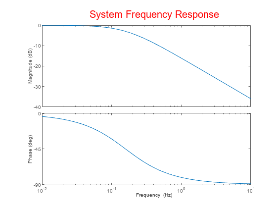
Because opts begins with a fixed set of options, the plot result is independent of the toolbox preferences of the MATLAB session.

Create a Bode plot that suppresses the phase plot and uses frequency units Hz instead of the default radians/second. Otherwise, the plot uses the settings that are saved in the toolbox preferences.

First, create an options set based on the toolbox preferences.

opts = bodeoptions('cstprefs');

Change properties of the options set.

opts.PhaseVisible = 'off';
opts.FreqUnits = 'Hz';

Create a plot using the options.

h = bodeplot(tf(1,[1,1]),opts);

Figure contains an axes object. The axes object with ylabel Magnitude (dB) contains an object of type line. This object represents untitled1.

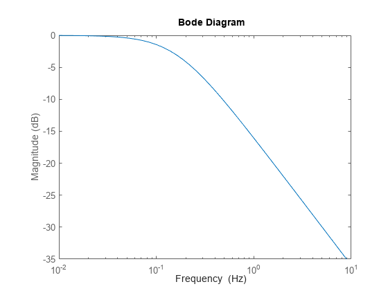
Depending on your own toolbox preferences, the plot you obtain might look different from this plot. Only the properties that you set explicitly, in this example PhaseVisible and FreqUnits, override the toolbox preferences.

Version History

Introduced in R2008a